Introduction

The hemodynamic response function (HRF) that describes the blood oxygenation level-dependent (BOLD) effect has been shown to vary in amplitude, timing, and shape across brain regions, cognitive states, with ageing, and pathology [1, 2]. Most efforts to characterize the BOLD response have focused on transient, task-evoked BOLD signals with known events or stimuli, because the timing information of spontaneous events in resting state for HRF estimation is not easily identified. Moreover, most measurements of the HRF have focused on gray matter (GM) as BOLD effects in white matter (WM) have been rarely reported [3] (and often are regressed out as nuisance covariates). WM in the brain is organized into distinct tracts that may be identified using diffusion MRI. This study aims to characterize the HRF in WM, its possible variation along white matter pathways, using resting state acquisitions. We aimed to quantify differences in HRF parameters between WM and GM, differences along WM pathways, and differences between WM pathways.

Methods

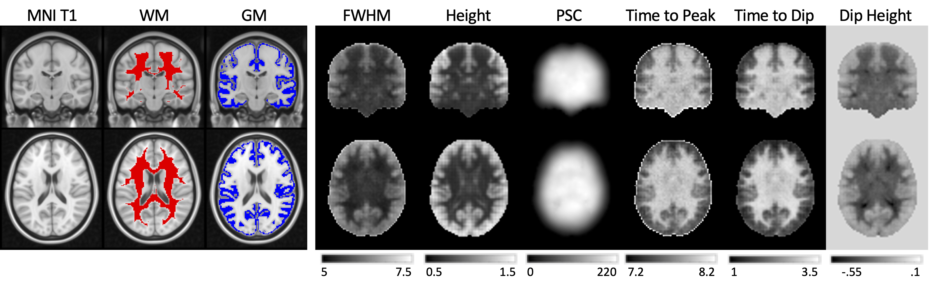
Data
199 subjects were randomly selected from the HCP S1200 release. Resting-state data were preprocessed using the minimal preprocessing pipelines described in [4],and non-linearly registered to MNI space after corrections for linear trends and temporal filtering with a band-pass filter (0.01-0.08 Hz). Strict WM and GM masks were derived from averaging WM/GM templates obtained from Freesurfer [5] across all subjects and thresholding at 0.9.
HRF estimation
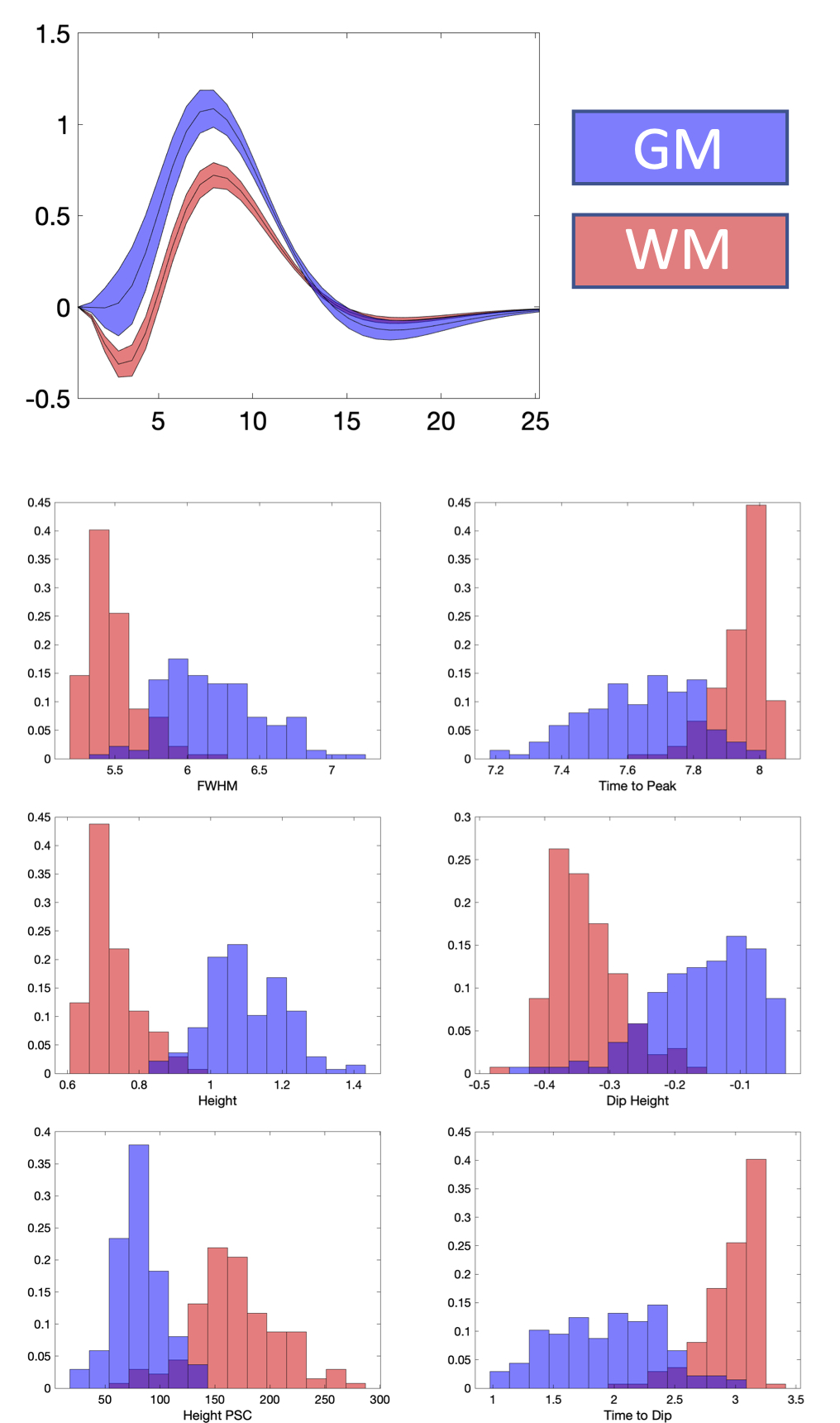
Voxel-wise HRFs were estimated using the rsHRF toolbox [6], which assumes that relatively large amplitude BOLD fluctuations can be identified and represent the occurrence of separable, spontaneous events. Following previous studies of WM HRFs [7], we used double-gamma functions together with a temporal derivative to fit the derived waveforms. This fitting incorporates an initial dip and time delay in the model response. Features of the HRF were then extracted for each voxel, including the full-width half maximum (FWHM, a metric of duration), peak height (Height), percent signal change (PSC), time to peak, time to dip, and initial dip height.
Along tract quantification
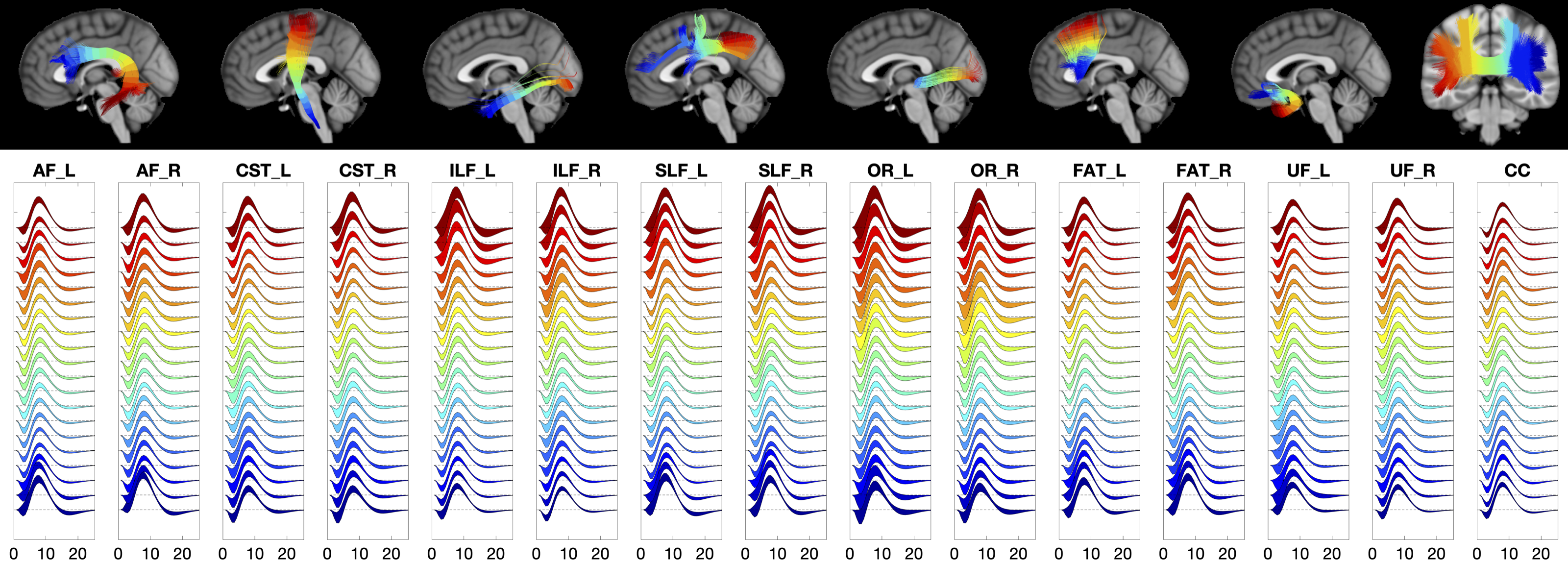
HRF features were quantified along major WM pathways using the along-fiber quantification technique on the population averaged WM tracts defined in [8]. Each pathway was segmented into N=20 points. Statistical analysis Linear mixed-effects modeling was used to ask whether HRF features change along pathways. y=β0+β1*position+β2*position²+β3*position³+β4(1|subject) where subjects were considered as a random effect, and we tested the null hypothesis that all fixed-effect coefficients equal zero (β1=β2=β3=0) using an F-test. A rejection of the null hypothesis suggests that a feature, y, changes along a pathway. We additionally performed a one-way analysis of variance to test for differences between pathways.

Results

What does the HRF look like averaged across a population?
Figure 1 shows WM and GM masks, and the 6 features of the HRF averaged across the population. WM and GM HRFs are qualitatively different, and all features show contrast between the tissues. Figure 2 quantifies differences in WM and GM HRFs. The GM HRF shows a typical canonical response, whereas the WM shows a consistent initial dip, and a smaller peak amplitude. The average WM HRF also has a shorter FWHM of the positive phase and longer time to peak, in agreement with previous literature.
What does the HRF look like within and along WM pathways?
The HRF for 15 WM pathways is shown in Figure 3. Here, streamlines are color coded from blue to red, with corresponding color-matched HRFs shown averaged across the population. Most notably, larger variations are observed near the WM/GM boundary at the ends of the pathway, with smooth trends along pathways.
Does the HRF change along pathways?
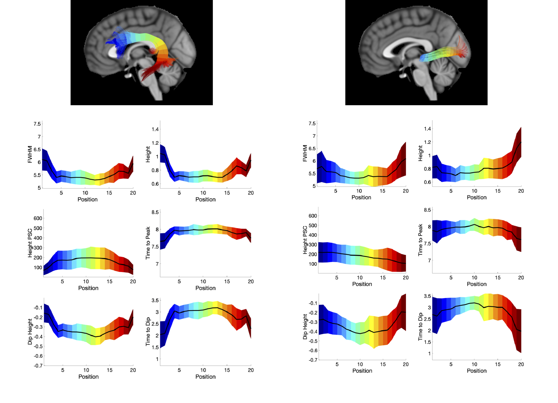
Figure 4 shows two exemplar pathways (the arcuate-fasciculus and optic-radiations) and the corresponding change in HRF features along the pathway. Trends are apparent along pathways, including a decreasing FWHM of the positive phase, height, and larger negative dip and increased time to peak in the middle core of the pathway. Statistical analysis confirms that all features, of all pathways, significantly change along the pathway from start to end.
Is the HRF different between pathways?
We aimed to extract a measure of changes in each HRF feature along pathways by taking the ratio of the range of that feature over the maximum value, calling this “% variation”. We find that several pathways show more variation in HRF features than others (Figure 5), including optic-radiations, and arcuate-fasciculi, and that the observed variations are significantly different across all pathways.

Discussion

We characterized the HRF of resting state fMRI within and across WM pathways. We created population-averaged maps of the HRF and its features, and show that, following major transient changes in resting state signal, WM responses have smaller peaks, are slower to change, and feature a prominent negative initial dip. Features of the HRF change significantly along WM pathways, and are much different in the deep WM than at the superficial WM. The variation observed along pathways also differs between pathways. Together, this suggests that, much like in GM, changes in flow and/or oxygenation related to variations in baseline conditions are different for different parts of the WM. These differences in HRF features may be relevant for understanding the biophysical basis of BOLD effects in WM.

Acknowledgements

This work was supported by the National Institutes of Health (NIH) grant R01 NS093669 (J.C.G), R01 NS113832 (J.C.G), R01EB017230 (B.A.L) and in part by ViSE (Vanderbilt Institute for Surgery and Engineering Nashville, Tennessee)/VICTR (The Vanderbilt Institute for Clinical and Translational Research) VR3029 and the National Center for Research Resources, Grant UL1 RR024975-01.