0505
Ultra-high field done ultra-fast:Enhancing Wave-CAIPI using an single-axis insert head gradient
1Highfield research group, University Medical Center Utrecht, Utrecht, Netherlands, 2Delft University of Technology, Delft, Netherlands, 3Spinoza Centre for Neuroimaging, Amsterdam, Netherlands
Synopsis
Acceleration techniques like SENSE have enabled significant decreases in scan time, but the $$$G$$$-factor penalty on SNR limits attainable accelerations.
Wave-CAIPI lowers this $$$G$$$-factor by spreading aliasing and taking advantage of the coil sensitivity distributions. A high performance single-axis insert gradient is utilised to increase the attainable wave amplitudes and thereby increasing the effectivity of Wave-CAIPI.
Simulations and 7T phantom & in-vivo acquisitions show significant improvements in $$$G$$$-factor when using Wave-CAIPI, especially when utilizing the higher performance of the insert gradient.
Not only are the $$$G$$$-factors lower but also show increased spreading and lack hard edges, allowing for even faster acquisitions.
Introduction
In recent years, acceleration techniques like SENSE and GRAPPA have enabled significant decreases in scan time, but even with the advance of ultra-high field scanners and their increased SNR, the penalty on SNR from $$$\sqrt{R}$$$ and $$$G$$$-factor limit attainable accelerations.Improved methods like CAIPI, BPE and Wave-CAIPI1 have been developed that try to lower this $$$G$$$-factor by spreading aliasing over the FOV and taking advantage of the coil sensitivity distributions. Previous work has predicted that Wave-CAIPI can benefit from using a high-performance insert gradient2, even when it only contains a single axis3.
Purpose
To reduce the $$$G$$$-factor penalty on SNR in highly accelerated scans by utilising Wave-CAIPI on a high performance single-axis head insert gradient, thereby allowing for even faster acquisitions without compromising on quality.Methods
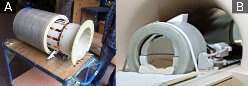
To study the effectivity of Wave-CAIPI with increased wave amplitudes on a single axis, simulations are performed and then validated in both phantom and in-vivo brain acquisitions on a 7T MRI scanner (Philips, Best, The Netherlands) with 32ch head coil (Nova Medical, Wilmington, USA).The chosen sequence is designed for SWI and consists of a whole-brain 3D GRE with a resolution of 0.8mm3 over a FOV of 256x192x256mm, with $$$T_{R}\mathrm{/}T_{E}\mathrm{/}α\mathrm{/}BW = 43\mathrm{[ms]/}20\mathrm{[ms]/}14°\mathrm{/}285\mathrm{[Hz]}$$$. The acquisition duration is reduced to 2min42sec by accelerating 16-fold, 4 times in both Y-& Z-axes, using SENSE and two types of Wave-CAIPI.
Wave-CAIPI is created by introducing a FOV/2 shift and 10 periods of sinusoidal waves on both Y-& Z-axes. The Z-axis wave is given a $$$90°$$$ phase offset to produce a cosine during the readout. The whole-body gradient specifications limit the wave amplitude to $$$9$$$ [mT/m] and that amplitude is therefore played out on the Y-axis.
The insert gradient produces the Z-axis wave and since previous work has shown that Wave-CAIPI efficiency improves with higher wave amplitudes4, the higher performance of the insert gradient is used to double the amplitude of the Z-axis wave to $$$18$$$ [mT/m] in the simulations and phantom acquisitions. To remain under auditory limits, a factor of 1.7x and thus $$$15.3$$$ [mT/m] waves are utilised in the in-vivo acquisitions. A secondary 1x reference acquisition is acquired for direct comparison with the higher performance waves.
Reconstruction is performed using an in-house developed NUFFT-based pipeline implemented in MATLAB complemented by MRecon (GyroTools, Zurich, Switzerland) and BART5. The real-time scanner behaviour and all resulting gradient waveforms are reproduced and convolved with a GIRF6 captured previously using a field camera7 (Skope, Zurich, Switzerland). For scans that just utilise the whole-body gradients the resulting trajectory suffices, but the insert gradient produces a B0 offset when not positioned perfectly on iso-center and therefore requires a PSF scan to measure and correct that offset. Sensitivity maps are calculated using ESPIRiT8 on a low-resolution reference acquisition. 18 iterations of CG-SENSE9 with $$$L_{2}$$$-regularisation produce the final reconstruction.
Simulations are created from a generated 3D phantom and acquired sensitivity maps. The phantom is multiplied by the sensitivities to produce ideal coil images. Noise is added to create a 14dB SNR and simulated K-space is calculated from those images using a NUFFT on trajectories taken from the reconstruction pipeline above.
Finally, G-factor maps are created for all reconstructions using the pseudo multiple replica method10 that performed the entire reconstruction 50 times with additional simulated noise.
Results
The $$$G$$$-factor analysis results for the simulations, phantom and in-vivo acquisitions that are depicted in figure 2 to 4 respectively, show a consistent pattern that is quantified in the table of figure 5.The Wave-CAIPI acquisition shows very significant reduction in $$$G$$$-factor over the SENSE acquisition. The enhanced (1.7x or 2x) Wave-CAIPI acquisition consistently improves over the regular Wave-CAIPI acquisition and shows even lower $$$G$$$-factor values.
The vendors SENSE implementation shows a similar pattern in $$$G$$$-factor to our SENSE implementation, but achieves slightly different results in which our implementation performs better on the phantom acquisition and the vendor SENSE shows favourable in-vivo $$$G$$$-factors.
Exemplar slices show slight folding artefacts in the SENSE acquisitions, which are not visible in the Wave-CAIPI acquisitions. However, the phantom Wave-CAIPI reconstructions show a ghost in the readout dimension that increases with increasing wave amplitude.
Discussion & Conclusion
Wave-CAIPI shows significant and consistent improvements in all acquisition types, not only are the absolute $$$G$$$-factor values themselves lower, they also show geometrical spreading and therefore lack the hard edges that frequently cause visible artefacts.The enhanced performance of the insert gradient enhanced the effect of Wave-CAIPI by further lowering the $$$G$$$-factor and increasing the spreading. The increase in wave amplitude slightly increased an artefact in the phantom acquisition, probably due to the higher sensitivity for imperfections in the trajectory and coil sensitivities produced by the pipeline that is tailored to in-vivo data. The chosen wave frequency limited the in-vivo capability of the gradient insert due to auditory limits, but that is reducible by changing frequency and could be completely eliminated by going above 20khz.
Conclusion
Wave-CAIPI significantly reduces the $$$G$$$-factor penalty on accelerated scans. While the high-performance single-axis insert head gradient shows clear improvements of the performance of Wave-CAIPI in the studied sequence, faster acquisitions are now feasonable (with increased R and shorter readouts, such as EPI) and have even larger potential performance benefits.Acknowledgements
No acknowledgement found.References
- Bilgic, Berkin, et al. "Wave‐CAIPI for highly accelerated 3D imaging." Magnetic resonance in medicine 73.6 (2015): 2152-2162.
- Versteeg, Edwin, et al. "A plug‐and‐play, lightweight, single‐axis gradient insert design for increasing spatiotemporal resolution in echo planar imaging‐based brain imaging." NMR in Biomedicine 34.6 (2021): e4499.
- Monreal Madrigal, Alejandro. "Ultra fast MRI acquisition at 7 Tesla: Implementation of Wave-CAIPI with a high efficiency head insert gradient coil." (2020).
- Wang, Haifeng, et al. "Parameter optimization framework on wave gradients of Wave‐CAIPI imaging." Magnetic resonance in medicine 83.5 (2020): 1659-1672.
- Uecker M, Ong F, Tamir JI, et al. Berkeley Advanced Reconstruction Toolbox. Annual Meeting ISMRM, Toronto 2015, In: Proc. Intl. Soc. Mag. Reson. Med 2015;23:2486.
- Vannesjo, Signe J., et al. "Gradient system characterization by impulse response measurements with a dynamic field camera." Magnetic resonance in medicine 69.2 (2013): 583-593.
- Wilm, Bertram J., et al. "Higher order reconstruction for MRI in the presence of spatiotemporal field perturbations." Magnetic resonance in medicine 65.6 (2011): 1690-1701.
- Uecker, Martin, et al. "ESPIRiT—an eigenvalue approach to autocalibrating parallel MRI: where SENSE meets GRAPPA." Magnetic resonance in medicine 71.3 (2014): 990-1001.
- Pruessmann, Klaas P., et al. "Advances in sensitivity encoding with arbitrary k‐space trajectories." Magnetic Resonance in Medicine: An Official Journal of the International Society for Magnetic Resonance in Medicine 46.4 (2001): 638-651.
- Robson, Philip M., et al. "Comprehensive quantification of signal‐to‐noise ratio and g‐factor for image‐based and k‐space‐based parallel imaging reconstructions." Magnetic Resonance in Medicine: An Official Journal of the International Society for Magnetic Resonance in Medicine 60.4 (2008): 895-907.
Figures
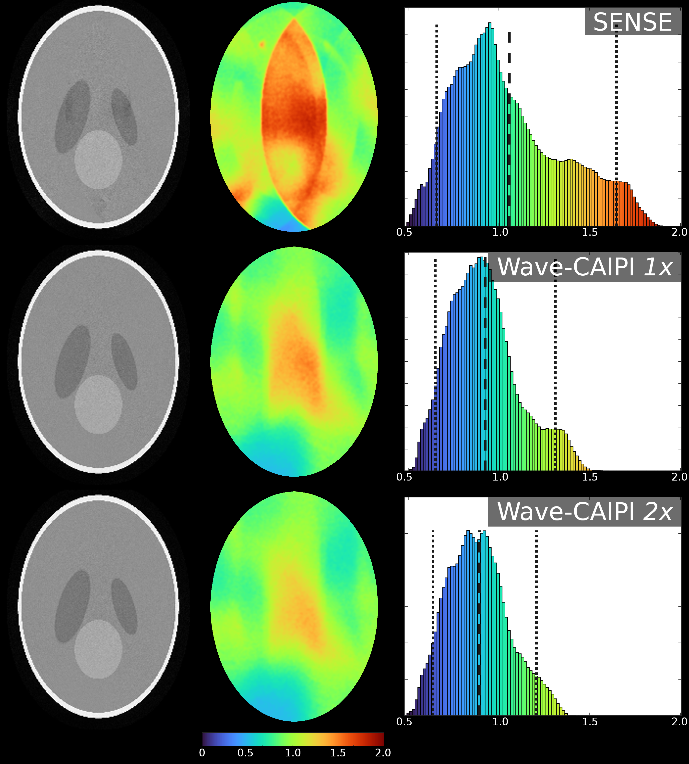
Results of the simulations for three types of acquisitions; SENSE, Wave-CAIPI 1x & Wave-CAIPI 2x from top to bottom, as marked in the figure.
The 2x acquisition utilises the higher performance available with the insert gradient and doubles the Z-axis waves over the 1x acquisition.
The left column depicts an exemplar image slice, the middle column the G-factors over that slice with colorbar below and the right column contains the histogram of G-factors from the entire 3D volume.
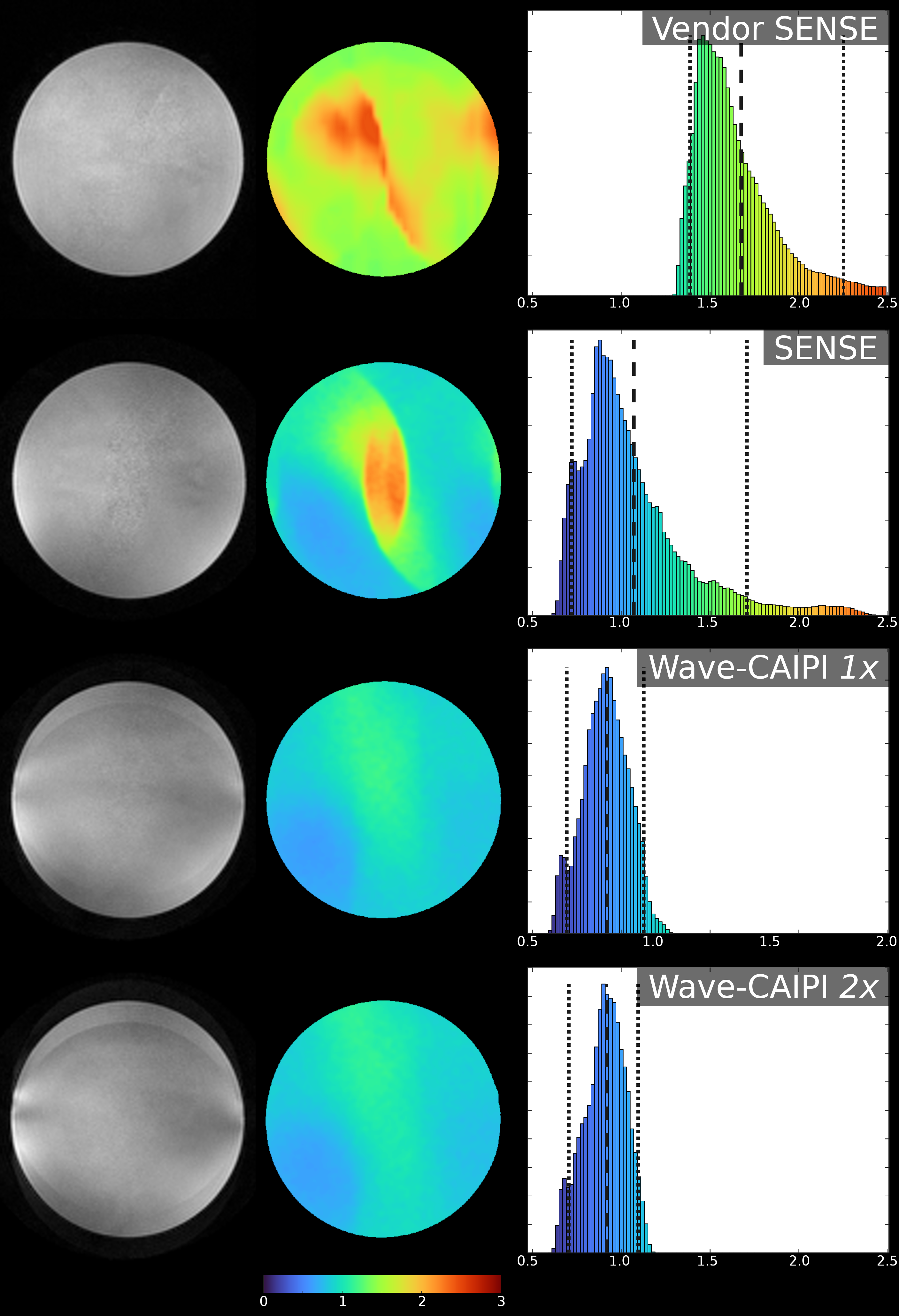
Results of the phantom acquisitions for four types of acquisitions; Vendor SENSE, SENSE, Wave-CAIPI 1x & Wave-CAIPI 2x from top to bottom, as marked in the figure.
The 2x acquisition utilises the higher performance available with the insert gradient and doubles the Z-axis waves over the 1x acquisition.
The left column depicts an exemplar image slice, the middle column the G-factors over that slice with colorbar below and the right column contains the histogram of G-factors from the entire 3D volume.
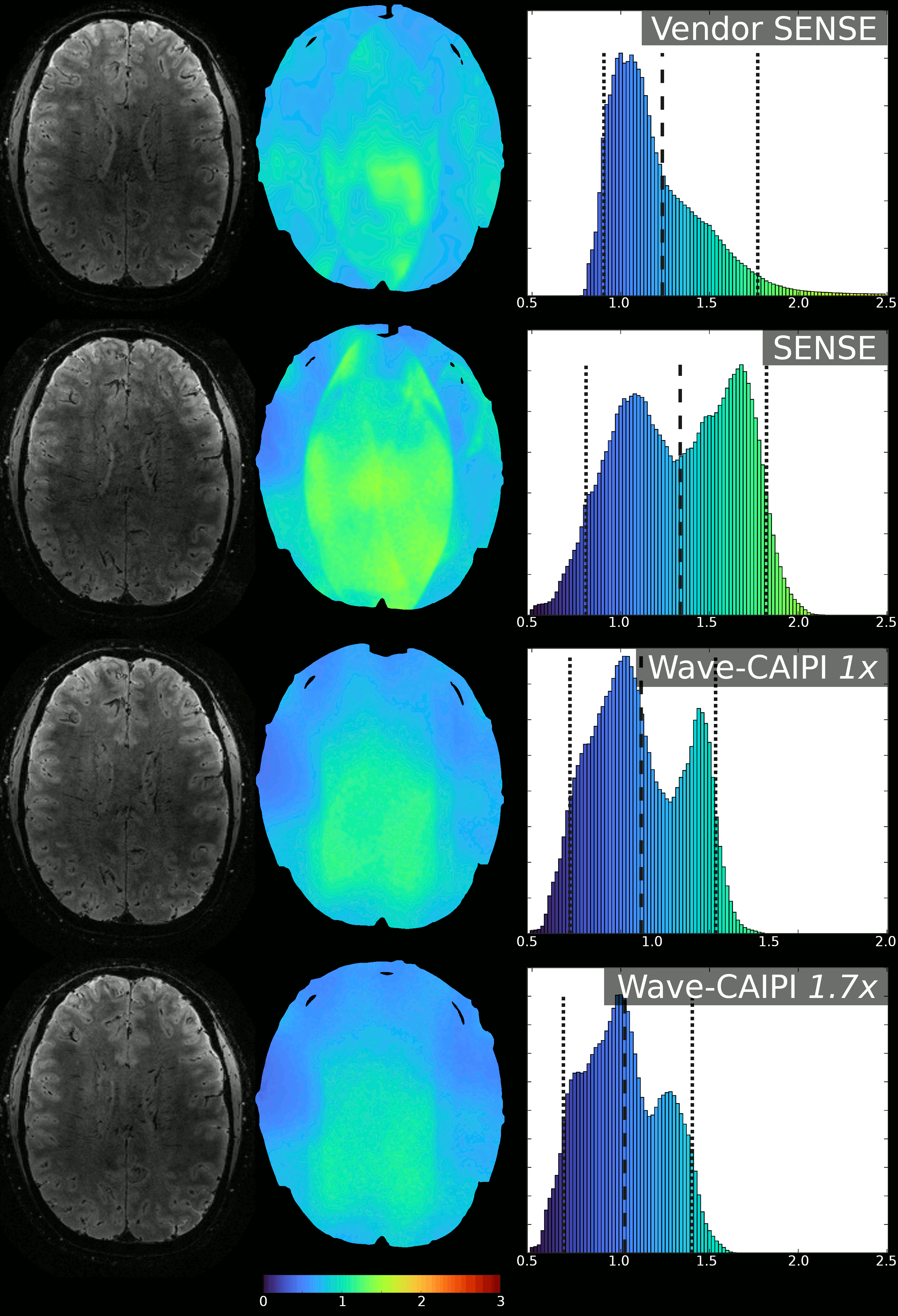
Results of the in-vivo acquisitions for four types of acquisitions; Vendor SENSE, SENSE, Wave-CAIPI 1x & Wave-CAIPI 1.7x from top to bottom, as marked in the figure.
The 1.7x acquisition utilises the higher performance available with the insert gradient and increases the Z-axis waves over the 1x acquisition.
The left column depicts an exemplar image slice, the middle column the G-factors over that slice with colorbar below and the right column contains the histogram of G-factors from the entire 3D volume.

Table with quantified results of G-factor analysis from all types of simulations, phantom & in-vivo acquisitions.
The three depicted metrics are the 5th percentile, mean and 95th percentile of G-factor values taken over their entire respective 3D volume. Each metric is also shown as a percentage change from the (vendor) SENSE acquisition.