Purpose

A critical measure of the performance of an imaging reconstruction is its noise propagation. However, the analytical computation of noise¹ becomes difficult for complex models, e.g., when non-linear regularizations are used, and the noise performance is often determined using Monte-Carlo simulations^2,3. Recent reconstruction approaches commonly involve neural networks (NNs) to solve the inverse problem^4–6. The advantage of NNs is that trained networks are generally non-iterative and computationally efficient; however, NNs intrinsically represent non-linear functions and consequently solutions may be unstable. We propose to estimate the noise propagation of NN-based reconstructions using automated differentiation⁷, which allows efficient calculation of the Jacobian matrix of the output with respect to the input.

Methods

E2E-VarNet: We studied the estimation of noise propagation of the end-to-end variational neural network (E2E-VarNet) to reconstruct uniformly under-sampled data. The E2E-VarNet imitates the steps of gradient descent algorithm which solves:
$$\hat{x}=argmin_{x}\frac{1}{2}||A\mathbf{x}-\mathbf{k}||^2+\lambda\Psi(\mathbf{x})\tag{1}$$
where x is vectorized coil-combined image, A is the encoding matrix to convert x into its vectorized k-space data k, and Ψ(x) is a regularization term. The gradient descent step is:
$$\mathbf{x}^{t+1}=\mathbf{x}^{t}-\eta^{t}A^{*}(A\mathbf{x}-\mathbf{k})+\lambda\Phi(\mathbf{x}^{t}) \tag{2}$$
where x^t denotes the value of x after iteration t with step size η^t, and Φ(x^t) is the derivative of ψ(x^t) with respect to x^t. The E2E-VarNet uses a cascade to imitate each gradient descent step:
$$\mathbf{k}^{t+1}=\mathbf{k}^{t}-\eta^{t}M(\mathbf{k}^t-\mathbf{k})+G(\mathbf{k}^{t})\tag{3}$$
k^t is the k-space after iteration t, M represents the sampling mask. G(k^t) is an operation involving two U-Net⁸ structures and performs functions resembling that of Φ(x^t) in Eq.2.
The E2E-Varnet used⁴ had 12 cascades and was pretrained with fast-MRI multi-coil brain data⁹ . Noise propagation was estimated using the 2D multi-coil brain test dataset acquired on 3 and 1.5T scanners, with T1-weighted or T2-weighted or FLAIR contrast (640x320 matrix). The image used in this work was uniformly under-sampled 11-fold, with a fully-sampled auto-calibration region of 24 lines.

Noise Propagation and Automated Differentiation: The theoretical noise propagation was derived from the Jacobian $$$J=\frac{∂\mathbf{I}}{∂\mathbf{K}}$$$ of the E2E-VarNet, where I was a reconstructed image and K the corresponding multi-coil single-slice k-space. J was calculated using automated differentiation⁷ which can accurately calculate derivatives by recording all operations in the computation of a scalar value of a function. The derivative of the function can then be calculated recursively based on the recorded operations.
To calculate the variance of the reconstructed image, we used a linear model to approximate the reconstruction from a noisy k-space vector:
$$\hat{\mathbf{I}}=\mathbf{I}+J\Delta\mathbf{k}\tag{4}$$
I is a noise-free image (vectorized) with k-space k. Δk is the noise in acquired k-space and Î denotes the reconstructed image from k-space k+Δk. If Δk is modeled as Gaussian noise with zero mean and covariance matrix W, the covariance of Î is:
$$Cov(\hat{\mathbf{I}})=\mathbf{J}W\mathbf{J}^{T}\tag{5}$$
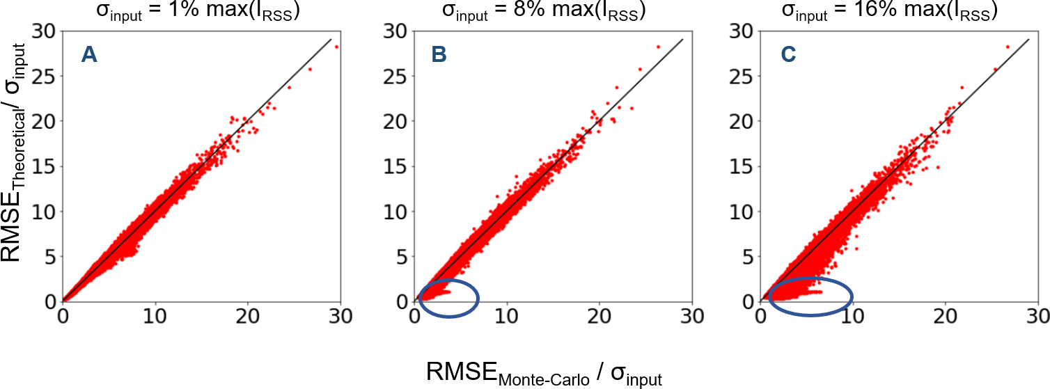
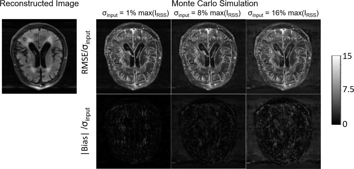
We used Eq.5 to calculate the noise propagation and compared it with Monte-Carlo Simulations, using the root-mean-square error (RMSE) of each voxel in the reconstructed image (normalized by dividing RMSE by input noise standard deviation σ). A square root of the sum of squares image was reconstructed (I_RSS) providing an intensity reference to the noise variance. Monte-Carlo simulations were performed with added noise of σ=1%max(IRSS), 8%max(IRSS), and 16%max(IRSS), each with 250 E2E-VarNet reconstructions.

Results

The reconstructed coil-combined image and sensitivity maps are presented in Figure 1. Voxel-wise RMSE of the output image in Monte-Carlo simulations normalized by the input σ are demonstrated in Figure 2 next to the theoretically calculated RMSE using automated differentiation. Overall, the theoretical calculation and Monte-Carlo simulation are in close agreement and difference maps (middle row) are close to 0. Figure 3 shows scatter plots of theoretical calculation versus Monte-Carlo simulation (RMSE). However, the difference increases with the input noise.
The absolute value of bias estimates and RMSE are compared side by side in Figure 4. The bias was almost negligible for σ=1%max(IRSS) and 8%max(IRSS), but becomes noticeable at 16%max(IRSS). Furthermore, the RMSE maps are spatially non-uniform, and noise magnification appears to be enhanced in areas with high intensity gradients in the input image (Figure 4).

Discussion

We were able to calculate theoretical noise propagation maps for the E2E-VarNet using automated differentiation. The resulting RMSE maps are in close agreement with those from Monte-Carlo simulations. Given the wide range of input noise intensities, these results suggest that the local linear model was an effective approximation for E2E-VarNet. The low bias level compared with the RMSE further supports the efficacy of this approximation and the proposed method. The linear approximation started to break down at relatively high noise levels [16%max(IRSS)], but these were higher than those typically encountered in clinical settings.
For purely linear reconstructions, the error caused by additive noise would be independent from the reconstructed image; however, the RMSE map appeared to be related to the spatial gradient of the reconstructed image. This correlation is likely caused by the non-linear component G(k) (Eq.5), i.e., the embedded NN, and the fact that the contribution of G(k) will heavily out-weigh the data consistency term (Eq.5) at the edge of k-space (but not in the fully-sampled central portion of k-space).
In conclusion, although further validation is required, the proposed method has great potential in estimating the noise propagation of image reconstruction techniques.

Acknowledgements

Radu Balan was supported in part by NSF grants DMS-1816608 and DMS-2108900 grants, and Thomas Ernst was supported by NIH grant 1R01 DA021146 (BRP).