0451

Pulsed Selective Excitation in Multiphoton MRI

Victor Han¹, Jianshu Chi¹, and Chunlei Liu^1,2
¹Electrical Engineering and Computer Sciences, University of California, Berkeley, Berkeley, CA, United States, ²Helen Wills Neuroscience Institute, University of California, Berkeley, Berkeley, CA, United States

Synopsis

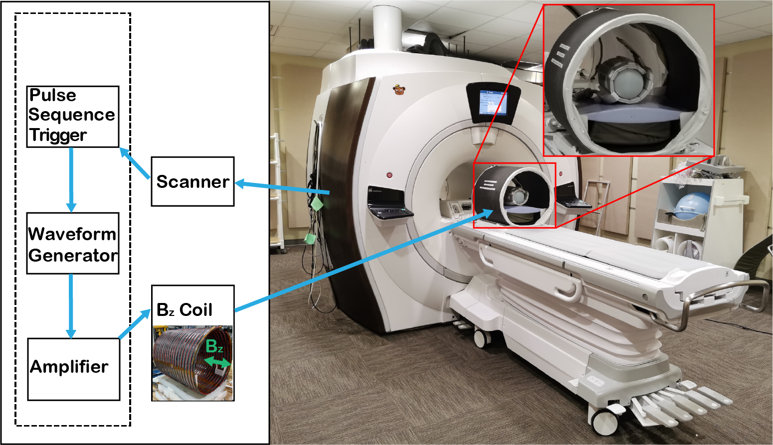
When multiple RF fields are applied at different frequencies, multiphoton excitation can occur when the sums or differences of integer multiples of these frequencies equal the Larmor frequency. No RF at the Larmor frequency is required. In this work, we describe the general principles of multiphoton pulsed selective excitation, providing a formalized treatment with design examples and implementations on a 3T scanner with an additional homemade z-direction (B_z) coil. With the additional B_z coil, we demonstrate additional flexibility, where the same excitation can be accomplished in several different ways with the same pulse duration.

Introduction

NMR excitation can occur not only at the Larmor frequency, but also at subharmonics of the Larmor frequency, a phenomenon called multiphoton excitation^1–3. Although subharmonic excitation at high $$$B_0$$$ fields is very inefficient, the efficiency can be greatly increased by using multiple frequencies to generate excitation instead of a single subharmonic. When multiple RF fields ($$$B_1$$$ fields) are applied at different frequencies, multiphoton excitation can occur when the sums or differences of integer multiples of these frequencies equal the Larmor frequency^4,5. With a proper choice of the RF frequencies, multiphoton excitation becomes practical in high-field MRI where SAR may be a concern.

In this work, we describe the general principles of multiphoton pulsed selective excitation, providing a formalized treatment with design examples and implementations on a 3T scanner with an additional homemade z-direction ($$$B_z$$$) coil. With the additional $$$B_z$$$ coil, we demonstrate additional flexibility, where the same excitation can be accomplished in several different ways with the same pulse duration.

Theory

With a small-tip angle approximation and ignoring relaxation, the Bloch equations can be written as
$$\begin{bmatrix}\dot{M_x}\\\dot{M_y}\end{bmatrix}=\gamma\begin{bmatrix}0&B_z(t)\\-B_z(t)&0\end{bmatrix}\begin{bmatrix}M_x\\M_y\end{bmatrix}+\gamma\begin{bmatrix}-B_y(t)M_0\\B_x(t)M_0\end{bmatrix}.\:\:\:[1]$$
Denote the transverse magnetization and magnetic field as
$$m_{xy}=M_x+iM_y,\:\:\:[2]$$
$$B_{xy}=B_x+iB_y.\:\:\:[3]$$
For pulsed B fields over the time period from 0 to T, the solution to Eq. [1] is given by
$$m_{xy}(\textbf{r},T)=i\gamma M_0\int_0^TB_{xy}(\textbf{r},t)e^{-i\gamma\int_t^TB_z(\textbf{r},\tau)d\tau}dt.\:\:\:[4]$$
In the Larmor frequency rotating frame, let us define
$$B_z=B_{1,z}(t)\cos{(\omega_zt+\phi)}+\textbf{G}\cdot\textbf{r},\:\:\:[5]$$
$$B_{xy}=B_{1,xy}(t)e^{-i((\omega_{xy}-\omega_0)t+\theta(t))}.\:\:\:[6]$$
These are the typical fields in MRI, except with the addition of a uniform RF field in the z-direction for multiphoton excitation. When the frequency of the xy-RF is far off from the Larmor frequency, but satisfies the multiphoton resonance condition $$$\omega_{xy}-\omega_0=n\omega_z$$$⁶, Eq. [4] can be rewritten as
$$m_{xy}(\textbf{r},T)=i\gamma M_0\int_0^TB_{1,xy}(t)e^{-i(n\omega_zt+\theta(t))}e^{-i\gamma\int_t^TB_{1,z}(\tau)\cos{(\omega_z\tau+\phi)}d\tau}e^{i\textbf{k}(t)\cdot\textbf{r}}dt,\:\:\:[7]$$
where $$$-\gamma\int_t^T\textbf{G}(\tau)d\tau=\textbf{k}(t)$$$ as in excitation k-space⁷.
If $$$B_{1,z}(\tau)$$$ is slowly varying compared to $$$\cos{(\omega_{1,z}\tau+\phi)}$$$, then the integral of their product is approximately the product of $$$B_{1,z}(\tau)$$$ and the integral of $$$\cos{(\omega_{1,z}\tau+\phi)}$$$. With this assumption, and using the Jacobi-Anger expansion shown below, where $$$J_m(-)$$$ is the Bessel function of the first kind of order m,
$$e^{i\frac{\gamma B_{1,z}}{\omega_z}\sin{(\omega_zt+\phi)}}=\Sigma_{m=-\infty}^\infty J_m\left(\frac{\gamma B_{1,z}}{\omega_z}\right)e^{im(\omega_zt+\phi)},\:\:\:[8]$$
Eq. [7] can be rewritten as
$$m_{xy}(\textbf{r},T)\approx i\gamma M_0\int_0^TB_{1,xy}(t)e^{-i(n\omega_zt+\theta(t))}\left(\Sigma_{m=-\infty}^\infty J_m\left(\frac{\gamma B_{1,z}(t)}{\omega_z}\right)e^{im(\omega_zt+\phi)}\right)e^{-i\frac{\gamma B_{1,z}(t)}{\omega_z}\sin{(\omega_zT+\phi)}}e^{i\textbf{k}(t)\cdot\textbf{r}}dt.\:\:\:[9]$$

Only the term with $$$m=n$$$ contributes significantly to the integral, giving
$$m_{xy}(\textbf{r},T)\approx i\gamma M_0\int_0^TB_{1,xy}(t)e^{-i\theta(t)}J_n\left(\frac{\gamma B_{1,z}(t)}{\omega_z}\right)e^{-i(\frac{\gamma B_{1,z}(t)}{\omega_z}\sin{(\omega_zT+\phi)}-n\phi)}e^{i\textbf{k}(t)\cdot\textbf{r}}dt.\:\:\:[10]$$
Eq. [10] shows that $$$B_{xy}$$$ and $$$B_z$$$ contribute to the excitation profile in a similar way with $$$B_{1,xy}(t)$$$ and $$$J_n\left(\frac{\gamma B_{1,z}(t)}{\omega_z}\right)$$$ available for amplitude modulation and $$$e^{-i\theta(t)}$$$ and $$$ e^{-i(\frac{\gamma B_{1,z}(t)}{\omega_z}\sin{(\omega_zT+\phi)}-n\phi)}$$$ available for phase modulation. This contrasts with the standard one-photon case where we would just have $$$m_{xy}(\textbf{r},T)\approx i\gamma M_0\int_0^TB_{1,xy}(t)e^{-i\theta(t)} e^{i\textbf{k}(t)\cdot\textbf{r}}dt$$$.

Methods

To demonstrate the principles described in the theory, we simulated and implemented three sets of related pulses. To generate each pulse, the following procedure was followed.

1. Generate a prototype pulse using a conventional method like the SLR algorithm⁸.
2. If designing a standard one-photon pulse, directly set $$$B_{xy}$$$ to the prototype pulse and finish.
3. Else if designing a multiphoton pulse, choose $$$\omega_z$$$.

Based on Eq. [10], choose values such that $$$B_{1,xy}(t)J_n\left(\frac{\gamma B_{1,z}(t)}{\omega_z}\right)$$$ equals the amplitude modulation of the prototype pulse, and $$$e^{-i\theta(t)}e^{-i(\frac{\gamma B_{1,z}(t)}{\omega_z}\sin{(\omega_zT+\phi)}-n\phi)}$$$ equals the frequency modulation of the prototype pulse. For multiphoton excitation, we have more variables to choose which can together achieve the same effects as in the one-photon case.
Shift the center frequency of the $$$B_{xy}$$$ pulse by $$$n\omega_z$$$.

Base SLR prototype pulses were generated using SigPy.RF⁹. See https://github.com/LiuCLab/multiphoton-selective-excitation for complete details on pulse generation. $$$\omega_z/(2 \pi)=25$$$ kHz for all experiments.

Results

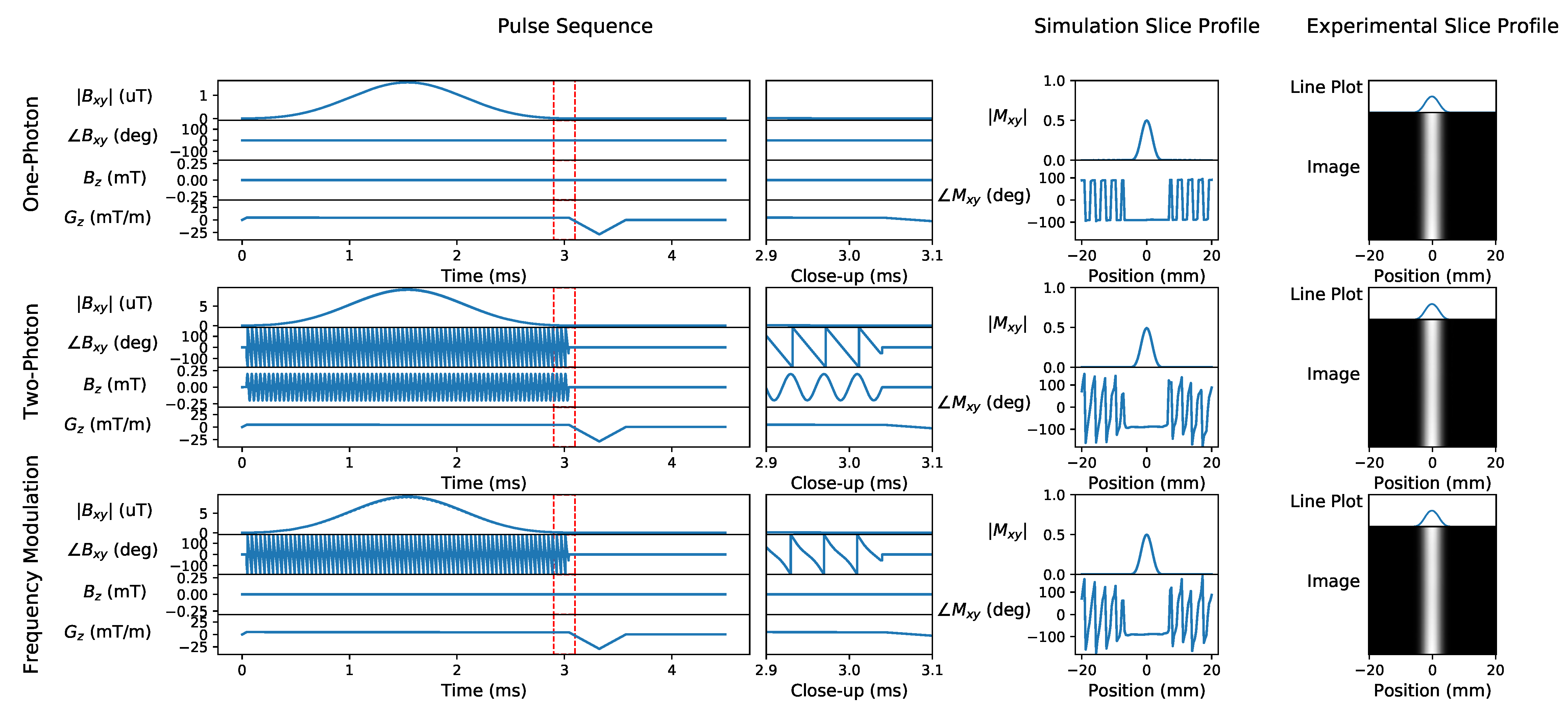
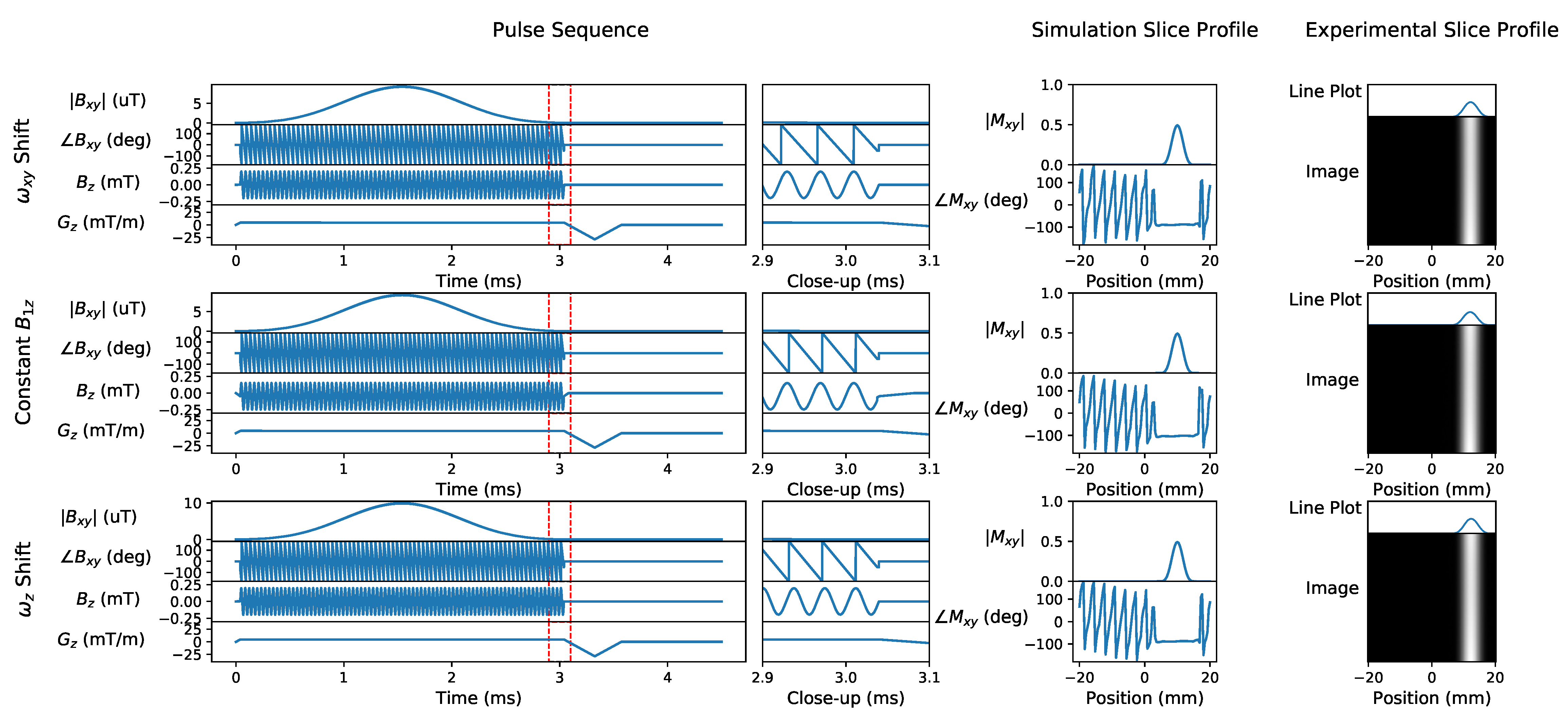
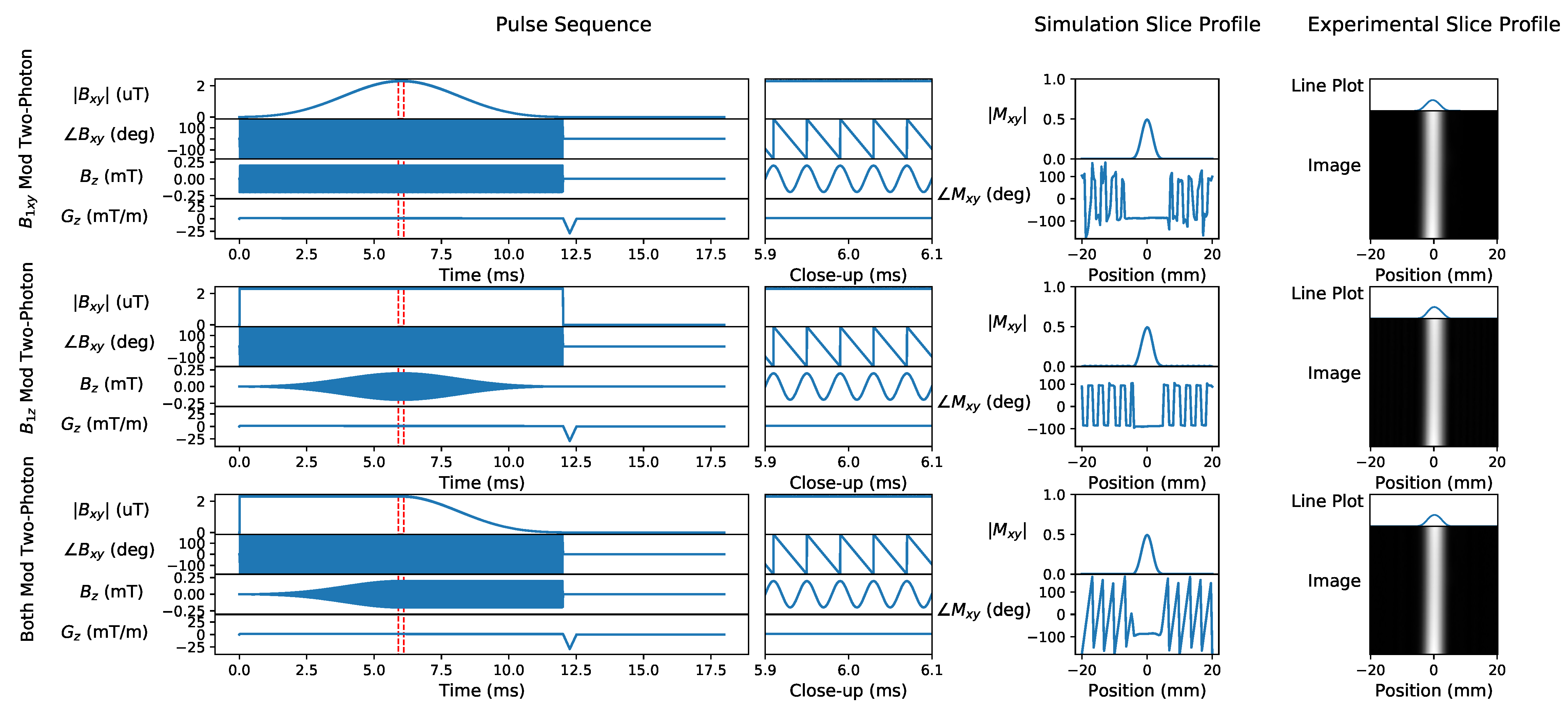
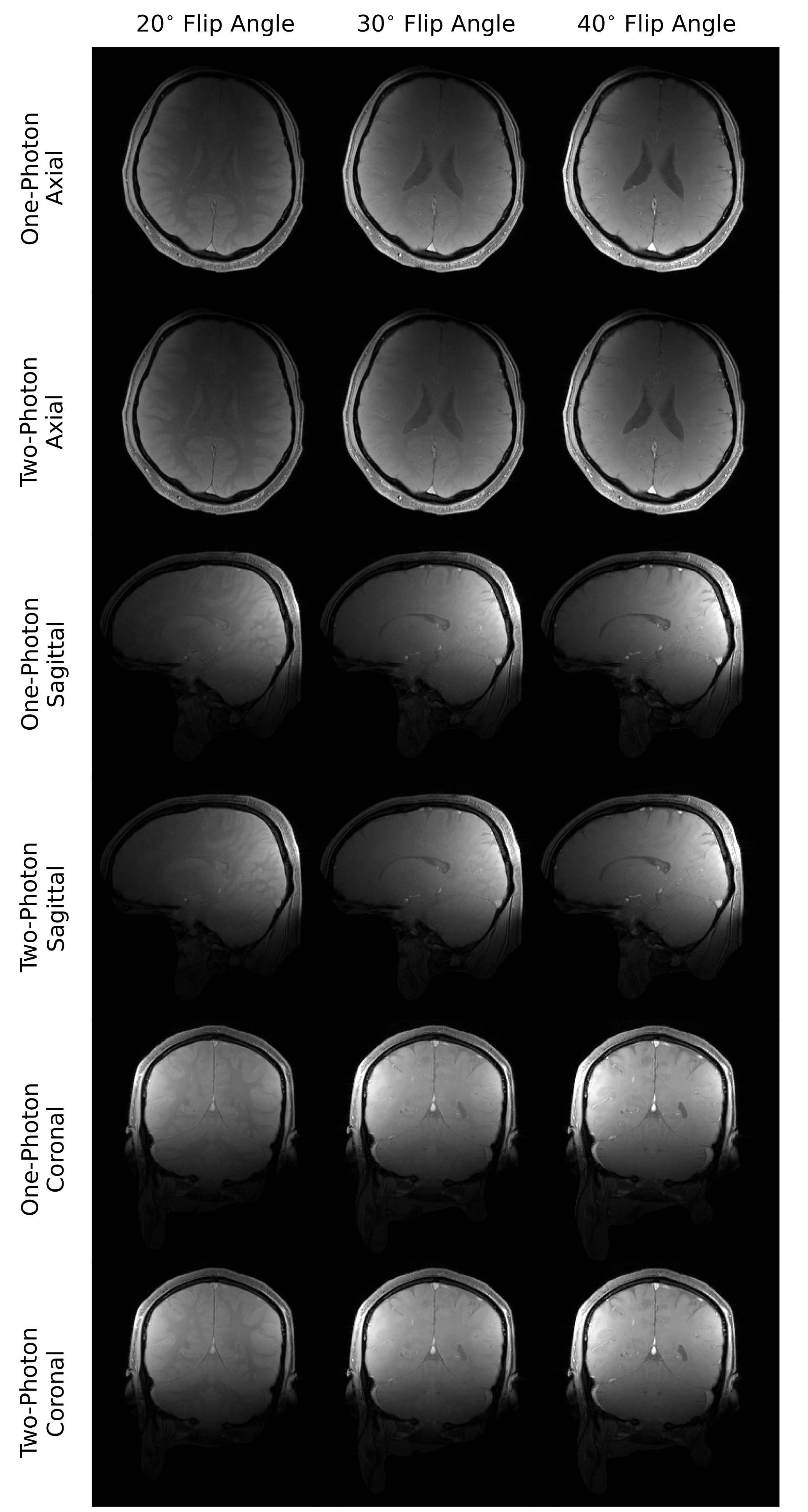
Fig. 1 shows the setup using an additional $$$B_z$$$ coil. Fig. 2 shows the simulations and experimental results of one-photon, two-photon, and frequency-modulated one-photon pulses producing the same slice selective excitation when designed to be equivalent. Frequency-modulated one-photon pulses are pulses which use $$$e^{-i\theta(t)}$$$ to imitate the effects of a $$$B_z$$$ pulse. Fig. 3 shows the two-photon pulse from Fig. 2, except shifted in position by three different methods. In Fig. 4, two-photon SLR pulses are demonstrated where the first pulse has amplitude modulation fully in the $$$B_{xy}$$$ pulse, the second pulse has amplitude modulation fully in the $$$B_z$$$ pulse, and the third pulse has amplitude modulation in both the $$$B_{xy}$$$ and $$$B_z$$$ pulses.

Using the same one-photon and two-photon pulses as in Fig. 2, Fig. 5 shows the in-plane results of the one-photon and two-photon pulses in vivo under our institution's IRB approval. No significant differences between the images are observed for this set of parameters.

Discussion and Conclusions

When $$$\omega_z$$$ is large enough, the distinction between the xy- and z-direction RF becomes smaller, and the ability to modulate $$$B_z$$$ instead of $$$B_{xy}$$$ gives extra flexibility to the multiphoton RF designer. We demonstrated how the same slice profiles can be achieved in many ways. Although not explored here, the principles of using a $$$B_z$$$ field for selective excitation could be extended to the use of arrays of z-direction coils for improving excitation homogeneity or tailoring excitation in general. Especially for low-field scanners where SAR is less of a concern, more eclectic applications can also be envisioned. For example, the traditional xy-RF transmit chain could be simplified in favor of a lower frequency z-RF. Alternatively, since the multiphoton pulses do not have any RF at the Larmor frequency, a pulsed version of simultaneous transmit and receive like in^10,11 could be implemented.

Acknowledgements

The authors thank Ekin Karasan and Miki Lustig for an introduction to HeartVista, Anita Flynn for improving lab spaces, and Karthik Gopalan for help and advice with mechanical engineering. This work was supported in part by NIH grant R21EB030157.

References

1. Eles PT, Michal CA. Two-photon excitation in nuclear magnetic and quadrupole resonance. Progress in Nuclear Magnetic Resonance Spectroscopy. 2010;56(3):232-246. doi:10.1016/j.pnmrs.2009.12.002

2. Michal CA. Nuclear magnetic resonance noise spectroscopy using two-photon excitation. The Journal of Chemical Physics. 2003;118(8):3451-3454. doi:10.1063/1.1553758

3. Abragam A. The Principles of Nuclear Magnetism. Clarendon Press; 1961.

4. Eles PT, Michal CA. Two-photon two-color nuclear magnetic resonance. The Journal of Chemical Physics. 2004;121(20):10167-10173. doi:10.1063/1.1808697

5. Zur Y, Levitt MH, Vega S. Multiphoton NMR spectroscopy on a spin system with I =1/2. The Journal of Chemical Physics. 1983;78(9):5293-5310. doi:10.1063/1.445483

6. Han V, Liu C. Multiphoton magnetic resonance in imaging: A classical description and implementation. Magnetic Resonance in Medicine. 2020;84(3):1184-119

7. doi:https://doi.org/10.1002/mrm.281867. Pauly J, Nishimura D, Macovski A. A k-space analysis of small-tip-angle excitation. Journal of Magnetic Resonance (1969). 1989;81(1):43-56. doi:10.1016/0022-2364(89)90265-5

8. Pauly J, Roux PL, Nishimura D, Macovski A. Parameter relations for the Shinnar-Le Roux selective excitation pulse design algorithm (NMR imaging). IEEE Transactions on Medical Imaging. 1991;10(1):53-65. doi:10.1109/42.75611

9. Martin J, Ong F, Ma J, Tamir J, Lustig M, Grissom W. SigPy.RF: Comprehensive Open-Source RF Pulse Design Tools for Reproducible Research. Proceedings of the ISMRM Annual Meeting and Exhibition. Published online 2020:1045.

10. Brunner DO, Pavan M, Dietrich B, Rothmund D, Heller A, Pruessmann K. Sideband Excitation for Concurrent RF Transmission and Reception. Proceedings of the ISMRM Annual Meeting and Exhibition. Published online 2011:625.

11. Brunner DO, Dietrich BE, Pavan M, Prüssmann KP. MRI with Sideband Excitation: Application to Continuous SWIFT. Proceedings of the ISMRM Annual Meeting and Exhibition. Published online 2012:150.

Figures

Fig. 1 – MRI System Setup with a $$$B_z$$$ Coil. For experiments that need a uniform $$$B_z$$$ field, the pulse sequence triggers a waveform generator. The output of the waveform generator gets amplified by an amplifier in voltage-controlled current mode, and the current goes to a big solenoid, which produces a magnetic field in the same direction as $$$B_0$$$. A smaller picture of the solenoid before it was encased is shown on the left. A knee coil for reception wraps arounds a phantom inside the solenoid. The body coil is used for $$$B_{xy}$$$ transmit.

Fig. 2 – Waveforms, Simulations, and Results for Corresponding One-photon, Two-photon, and Frequency Modulation Pulses. The excitation pulse sequence, simulation, and experimental results are shown for corresponding one-photon, two-photon, and frequency modulated one-photon pulses. The dotted red lines indicate where the close-up view of the pulse sequence is. All pulses are 5 mm slice thickness and have a time-bandwidth product of 3. The profiles are the same in both simulation and experiment.

Fig. 3 – Waveforms, Simulations, and Results for Corresponding Slice Position Shifts with $$$\omega_{xy}$$$, Constant $$$B_z$$$, or $$$\omega_z$$$. The excitation pulse sequence, simulation, and experimental results are shown for equivalent slice shifts using a change in $$$\omega_{xy}$$$, a DC $$$B_z$$$ field, and a change in $$$\omega_z$$$. From the close-ups, the first pulse has a slightly slower $$$B_{xy}$$$ phase variation, the second pulse has a slight negative DC offset with a ramp at the end in the $$$B_z$$$ field, and the third pulse has a slightly higher $$$\omega_z$$$.

Fig. 4 – Waveforms, Simulations, and Results for Corresponding Pulses Using Modulation in $$$B_{1,xy}$$$, $$$B_{1,z}$$$, or Both. The excitation pulse sequence, simulation, and experimental results are shown for equivalent two-photon pulses with modulation in $$$B_{1,xy}$$$, $$$B_{1,z}$$$, or both. With the longer pulse duration, the oscillations on $$$B_{1,z}$$$ are no longer easily visible, thus better satisfying the assumption that modulation on $$$B_{1,z}$$$ is slow compared to $$$\omega_z$$$. The dotted red lines indicate where the close-up view is.

Fig. 5 – In Vivo One- and Two- Photon Selective Excitations Produce Similar Images When Designed to be Equivalent. The same one- and two-photon selective excitation pulses from Fig. 2 were used for slice-selective in-plane imaging of a healthy volunteer. Three different orientations are shown for three different flip angles. The maximum flip angle was limited by the peak $$$B_{1,xy}$$$ amplitude required for the given pulse parameters and maximum $$$B_{1,z}$$$ amplitude available. The sagittal and coronal images were cropped to remove some empty space.

Proc. Intl. Soc. Mag. Reson. Med. 30 (2022)

0451

DOI: https://doi.org/10.58530/2022/0451