Synopsis

Streamlined qBOLD acquisitions enable experimentally straightforward observations of brain metabolism. High quality R2’ maps are easily derived; however, the oxygen extraction fraction (OEF) and deoxygenated blood volume (DBV) are more ambiguously defined from noisy data. Accordingly, standard approaches yield noisy and underestimated OEF maps and overestimate DBV.

This work uses synthetic data to learn models for voxelwise prior distributions, which are subsequently leveraged in an amortized variational Bayesian inference model. We demonstrate our approach enables inference of smooth OEF and DBV maps, with a physiologically realistic distribution, and illustrate voxelwise differences in OEF between subjects at rest and undergoing hyperventilations.

Introduction

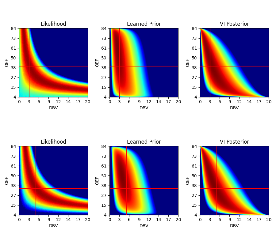
Quantitative blood oxygen level dependent (qBOLD) MRI provides a mechanism for creating in-vivo maps of brain metabolism¹. This finds application in the study of healthy brain physiology, as well as in several clinical applications ranging from stroke to dementia and other neurological diseases.
More recently, streamlined qBOLD acquisitions using asymmetric spin echo sequences² have provided experimentally straightforward observations of brain metabolism. Although this approach has been shown to yield high quality R2’ maps, the oxygen extraction fraction (OEF) and deoxygenated blood volume (DBV) have a complex joint distribution given the data, where a range of OEFs and DBVs are similarly probable (see Figure 1 left column). Maximum likelihood estimation yields unrealistic parameter ranges for both DBV and OEF, and extremely noisy OEF maps (see Figure 3, second column). Moreover, they (and previous Bayesian approaches³) utilise a linearised form of the signal model and predict OEF as a derived quantity, which complicates the use of priors.
We propose a novel probabilistic machine learning solution, based on amortized variational inference⁴, which estimates physiologically plausible and interpretable maps of the joint distribution of OEF and DBV from streamlined qBOLD data.

Methods

Our approach takes a two stage approach to creating an inference model, see figure 2 for an illustration. We first train a neural network with simulated data to predict the joint distribution of OEF and DBV. Subsequently, this synthetically trained model provides informative voxelwise priors for training an amortized variational inference model on real images.
We use a variant of the multivariate logit-Normal ($$$L\mathcal{N}$$$) distribution (pdf below) for the predicted OEF and DBV parameters to allow correlated parameters while limiting their range:
$$ f(\mathbf{y}; \mu_l, \Sigma_l) = \frac{1}{\sqrt{2\pi}|\Sigma^{\frac{1}{2}}|}\frac{1}{\sum_i^2 \mathbf{y}_i(1-\mathbf{y}_i)}\exp \left(-0.5(\mathrm{logit}(\mathbf{y})-\mu_l)^T\Sigma_l^{-1}(\mathrm{logit}(\mathbf{y})-\mu_l)\right) $$
As shown in figure 1 middle and right columns, this allows for a flexible description of the joint distribution.

Synthetic data was generated using the non-linear signal equation, $$$S_\tau(\mathrm{OEF}, \mathrm{DBV})$$$, where $$$\tau$$$ is the spin echo displacement time. Gaussian noise was added to each image to provide an SNR between 50-120. The synthetic OEFs and DBVs were sampled from reasonably narrow Normal distributions to induce a bias to a physiologically plausible range: $$$\mathrm{OEF}\sim \mathcal{N}(40\%, 20\%^2)$$$, $$$\mathrm{DBV}\sim\mathcal{N}(2.5\%, 2\%^2)$$$. The prior model was trained using the AdamW³ optimiser, with lr=2e^-3 and weight decay=2e^-4. As illustrated in figure 1, the prior is moderately informative and offers little support to low OEF/high DBV.
The amortized variational inference model learns to predict an approximate posterior distribution for OEF/DBV from real data. The loss function, given observed data $$$\mathbf{X}$$$, is the negative log evidence lower-bound (ELBO), which is defined below:
$$\mathcal{L} = - E_{q([OEF, DBV]|\mathbf{X})}\left[p(\mathbf{X} | [OEF, DBV])\right] + D_{KL}(q([OEF, DBV] | \mathbf{X}) || p([OEF, DBV]) $$
$$\approx - \sum_j^{N_s} \mathcal{N}(\mathbf{X}; S(\tau,[OEF, DBV]^j), \Sigma_{im})) + D_{KL}\left(L\mathcal{N}(\mu_{l,vi}, \Sigma_{l,vi}) || L\mathcal{N}(\mu_{l,p}, \Sigma_{l,p})\right), \mathrm{where} [OEF, DBV]^j\sim q([OEF, DBV]|\mathbf{X})$$
The ELBO of validation data was used for all hyper-parameter selection. To encourage additional spatial smoothness, we introduce a total variation regularisation on the predicted mean OEF/DBV. Although principled approaches exist to infer spatial regularisation⁶, these have not been demonstrated for multivariate logit-Normal distribution. The model is optimised using AdamW with lr=5e^-3 and weight decay 2e^-4 on random 25x25x8 crops. The data is normalised by dividing by the spin-echo volume and taking the logarithm.
The model architecture consists of 1x1x1 convolutions (to enable training on spatially independent synthetic data) as well as gated 3x3x1 convolutional blocks, which are additionally used when training on real images. We opt for 2 convolution blocks with 60 hidden units.

Data

All data were acquired with the FLAIR-GESEPI-ASE sequence described in², with an in-plane axial resolution of 96x96, with 8 slices. The voxel dimensions were 2.3mmx2.3mmx5mm, with a 2.5mm slice gap. For each acquisition, 11 values of $$$\tau$$$ were used, from -16ms to 64ms with an 8ms spacing.
The training dataset consisted of 22 subjects, some of which had repeated scans, covering: central, inferior or superior areas of the brain.
The validation dataset consisted of 5 healthy subjects, where data were acquired both at rest and when undergoing hyperventilation, monitored using capnography. During hyperventilation, OEF is expected to increase, in order to compensate for the increase in cerebral blood flow.

Results

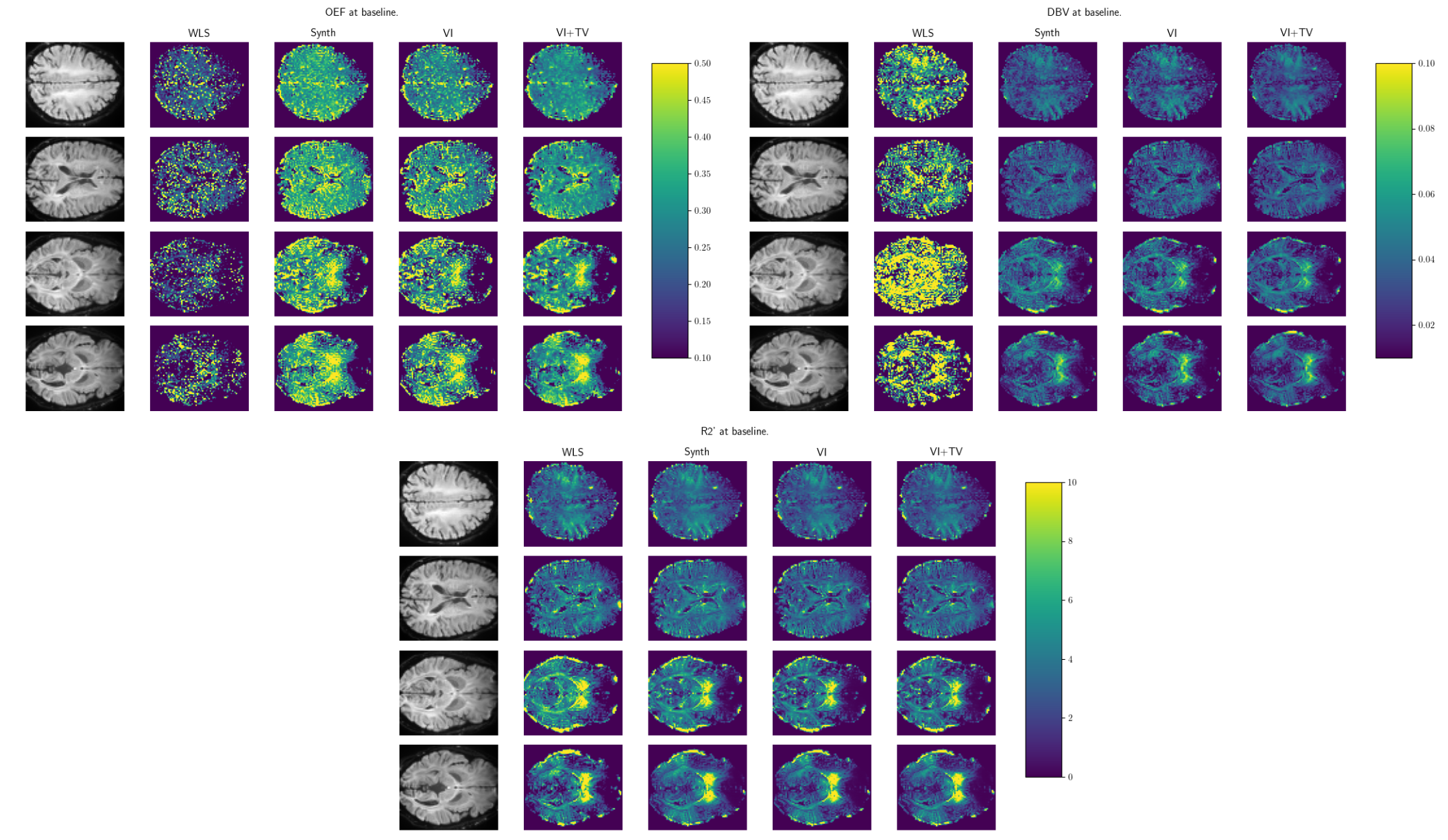
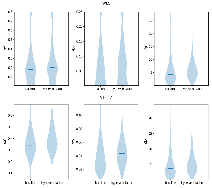
All results are reported on the validation dataset. Figure 3 provides some example parameter maps comparing our approach and weighted least squares (WLS). These illustrate that our approach yields substantially smoother and more interpretable OEF and DBV maps. Furthermore, we illustrate the inferred gray matter distributions from WLS and our approach in Figure 4, and observe clearer differences between baseline and hyperventilation. Figure 5 demonstrates a voxelwise statistical comparison where significant increases in OEF are observable with our proposed approach.

Discussion

We found that specifying a relatively tight distribution of OEF/DBV when training our prior model encourages our predicted parameters to lie within a more physiologically plausible range. Moreover, all the models trained to predict OEF/DBV directly produced cleaner maps.

Conclusion

The improved predictions from our model enables interpretable voxelwise measurement of OEF and DBV from streamlined qBOLD data. This may lead to wider adoption of such methods for analysing oxygenation. Future work will integrate this approach with cerebral blood flow measures to provide a more complete description of brain metabolism.

Acknowledgements

The University of Brighton Rising Stars initiative funded the acquisition of this data.