0373
Denoising and Uncertainty Estimation in parameter mapping With Bayesian Deep Image Prior
Max Hellström1 and Anders Garpebring1
1Radiation Sciences, Umeå University, Umeå, Sweden
1Radiation Sciences, Umeå University, Umeå, Sweden
Synopsis
Tissue parameter estimation often gives noisy parameter maps due to noise in the signal data. In this work, we improve parameter mapping by incorporating noise reduction and uncertainty estimation with Bayesian Deep Image Prior. We implement task-specific loss functions for different applications. We test our method by estimating T1, T2, and ADC with synthetic- and in-vivo MRI data. Our method results in denoised tissue parameter maps, with associated error estimates. Our method is easy to implement, does not require any training data, and is easy to customize for different applications in parameter mapping.
Introduction
The image contrast in Magnetic Resonance Imaging (MRI) depends on several tissue parameters of the imaged patient. Quantitative MRI is a subset of MRI that include actual quantification of these tissue parameters. These methods require a series of MRI images and a post-imaging reconstruction process that isolates the relationship between the MRI signal and the tissue parameters of interest in the imaged region. There are several medical applications where the quantification of tissue parameters provide useful information, e.g. in oncology1,2,3.The tissue parameter estimation (commonly referred to as parameter mapping) is a post-imaging procedure. Conventionally, the value of the tissue parameters is calculated by a pixel-wise non-linear least squares (NLLS) regression of the MRI magnitude signal data, which can result in noisy parameter maps. Adding denoising into this process introduces spatial correlations which makes uncertainty estimation more complicated. Convolutional neural networks (CNN) are capable to address spatial correlations, but these methods require large training datasets that are highly specific for each problem of interest. Blind denoising of image data with deep image prior4 (DIP) has been shown successfully in several applications, including medical imaging applications5,6,7. These methods are CNN based but do not require any training dataset which makes the methods easier to implement. Combining a DIP approach with uncertainty estimations, e.g., from a Bayesian approximation8, results in methods that address denoising and uncertainty estimation without the need for a training dataset. Here we extend this concept to parameter mapping in quantitative MRI by implementing task-specific loss functions.
Methods
In this work, we address parameter mapping with a convolutional neural network (CNN) based framework. With a parameter mapping dataset $$$\boldsymbol{y} \in \mathbb{R}^{V \times M}$$$, i.e., a total of $$$M$$$ magnitude signal measurement over $$$V$$$ voxels, we define task-specific loss functions$$E(\mathbf{y}; \boldsymbol{\beta}) = \frac{1}{VM}\sum_{v=1}^{V}\sum_{m=1}^{M}\Big\Vert y_{v,m} - s(t_m, \boldsymbol{\beta}_v) \Big\Vert_2^2$$
where $$$s$$$ is the magnitude MR signal equation, which depends on both scanner settings $$$t$$$ and the tissue parameters $$$\boldsymbol{\beta}$$$. Examples of applications are variable flip angle T1 estimation with spoiled gradient echo and multi-echo spin-echo for T2 estimation.
Following the works of Ulyanov4 et al, we define $$$\mathbf{f}_{\boldsymbol{\theta}}(\mathbf{Z})$$$ to be the output of a CNN $$$\mathbf{f}$$$ with weights $$$\boldsymbol{\theta}$$$, when given a random tensor $$$\mathbf{Z}$$$ as input. $$$\mathbf{f}$$$ is then reinterpreted as a Bayesian Neural Network with Bernoulli variation inference9 by appending dropout after every convolution layer. DIP-enhanced parameter mapping is then implemented by optimizing over network weights
$$\arg \min_\boldsymbol{\theta} \frac{1}{VM}\sum_{v=1}^{V}\sum_{m=1}^{M}\Big\Vert y_{v,m} - s(t_m, \mathbf{f}_{\boldsymbol{\theta}}(\mathbf{Z})_v) \Big\Vert_2^2,$$
and after a number of iterations, estimate the tissue parameters with Monte Carlo integration of $$$N$$$ concurrent forward passes with dropout applied
$$$\hat{\boldsymbol{\beta}} = \frac{1}{N}\sum_{n=1}^{N} \mathbf{f}_{\boldsymbol{\theta}}(\mathbf{Z})$$$ with associated model uncertainty $$$\sigma_{\hat{\boldsymbol{\beta}}} = \frac{1}{N}\sum_{n=1}^{N} (\mathbf{f}_{\boldsymbol{\theta}}(\mathbf{Z}) - \hat{\boldsymbol{\beta}})^2$$$. This enables noise-reduced parameter mapping with associated model uncertainty estimation, without explicitly formulated spatial priors nor task-specific training data sets.
Our method was tested with three separate parameter mapping tasks: Variable flip-angle spoiled gradient echo for T1 mapping, multi-echo spin-echo for T2 mapping, and spin-echo based diffusion imaging for ADC mapping. For all tests, a skip-connection U-net (with about $$$2.2\times 10^{6}$$$ trainable parameters) was selected as network architecture. The method was tested on both in-vivo data and synthetically generated MRI signal with ricean distributed noise and a known ground-truth reference.
This study was conducted in accordance with the principles embodied in the Declaration of Helsinki and was ethically approved by the regional research ethics committee (dnr: 2019-02666).
Results
Tissue parameter estimation with synthetic data is presented in figure 1 (T1 estimation with VFA data) and figure 2 (T2 estimation with multi-echo spin-echo data). In both cases, the result clearly illustrates the denoising feature of DIP with a decrease in root mean squared error, but even more important, that the concept of DIP denoising extend into the domain of parameter mapping in quantitative MRI. The added benefit of the Bayesian approximation is illustrated in figure 3, which highlights the sampling distribution of the T1 samples at different spatial locations.ADC mapping with in-vivo data is presented in figure 4, which gives similar results as in figure 1 and 2, but with no available ground truth reference.
Discussion and Conclusion
Our method successfully produces parameter maps with the added benefits of significant noise reduction and model uncertainty estimation. In contrast to conventional CNN approaches, our method does not require any training dataset due to the DIP implementation. Our method is easy to customize for different applications since the reconstruction is embedded in a loss function that is specific to the problem of interest, and the majority of the CNN architecture can be reused for different applications.Future work and further investigations should address computational efficiency, optimization stopping criterion, and uncertainty calibration.
Acknowledgements
This research was in part funded by grants from The Swedish Research Council (grant number 2019-0432), Region Västerbotten (Central ALF, grant number RV-738491), Cancerforskningsfonden i Norrland (grant number AMP 18-912), and Lions Cancerforskningsfond (grant number LP 18-2182).References
- Fütterer, J, Multiparametric MRI in the detection of clinically significant prostate cancer, Korean Journal of Radiology (2017),10.3348/kjr.2017.18.4.597
- CHAPTER 2 - Evaluation of the Symptomatic Patient: Diagnostic Breast Imaging. In Marie Tartar,Christopher E Comstock, and Michael S Kipper, editors, Breast Cancer Imaging, pages 38–75. Mosby,Philadelphia, 2008
- Mai J, et al. T2 Mapping in Prostate Cancer. Investigative Radiology, 54(3),1292019
- Ulyanov D, et al. Deep Image Prior. International Journal of Computer Vision, 128(7), 2020
- Jin, K. H., Gupta, H., Yerly, J., Stuber, M., & Unser, M. (2019). Time-dependent deep image prior for dynamic MRI. arXiv e-prints, arXiv-1910.
- Gong, K., Catana, C., Qi, J., & Li, Q. (2018). PET image reconstruction using deep image prior. IEEE transactions on medical imaging, 38(7), 1655-1665.
- Lin, Y. C., & Huang, H. M. (2020). Denoising of multi b-value diffusion-weighted MR images using deep image prior. Physics in Medicine & Biology, 65(10), 105003.
- Laves, M. H., Tölle, M., & Ortmaier, T. (2020). Uncertainty estimation in medical image denoising with bayesian deep image prior. In Uncertainty for Safe Utilization of Machine Learning in Medical Imaging, and Graphs in Biomedical Image Analysis (pp. 81-96). Springer, Cham.
- Gal Y, Ghahramani Z, Bayesian Convolutional Neural Networks with Bernoulli Approximate Variational Inference, 2015, arXiv:1506.02158
Figures
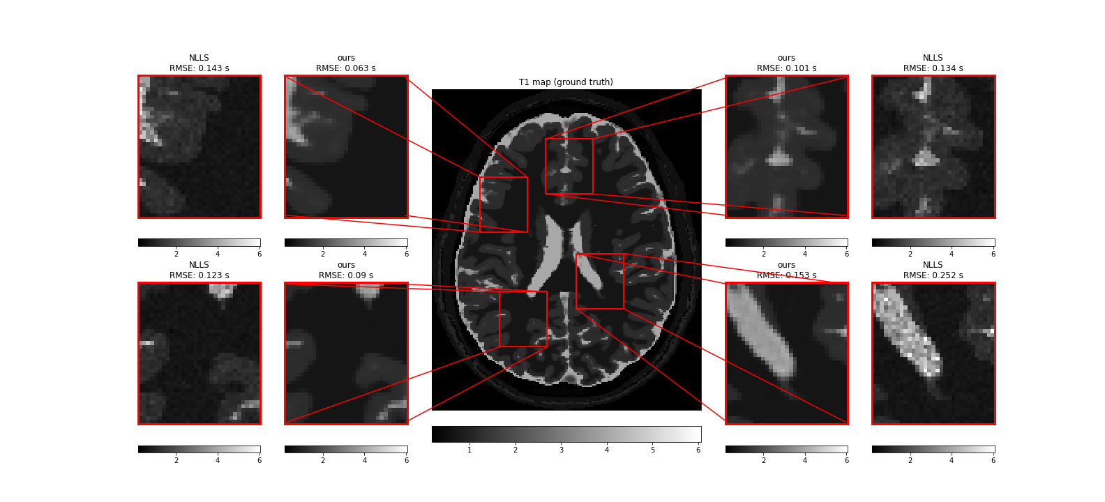
Comparison of T1 parameter map (in seconds) obtained with our method (mean image over 1280 samples, after 150k optimization steps), compared to conventional NLLS estimation. The centre image is the ground-truth reference. The synthetic MRI signal (SPGR) was generated from ground truth reference maps of T1 and proton density, with flip angles 2, 4, 11, 13, and 15 degrees, and a repetition time of 6.8 ms. For each of the four zoom regions, the root mean squared error (RMSE) was calculated with the ground truth as a reference.
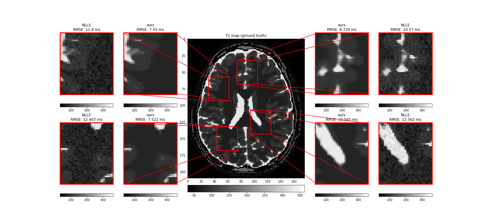
Comparison of T2 parameter map (in milliseconds) obtained with our method (mean image over 1280 samples, after 150k optimization steps), compared to conventional NLLS estimation. The centre image is the ground-truth reference. The synthetic MRI signal (multi-echo spin-echo) was generated from ground truth reference maps of T2 and proton density, with echo times 0.05, 0.15, and 0.3 seconds. For each of the four zoom regions, the root mean squared error (RMSE) was calculated with the ground truth as a reference.
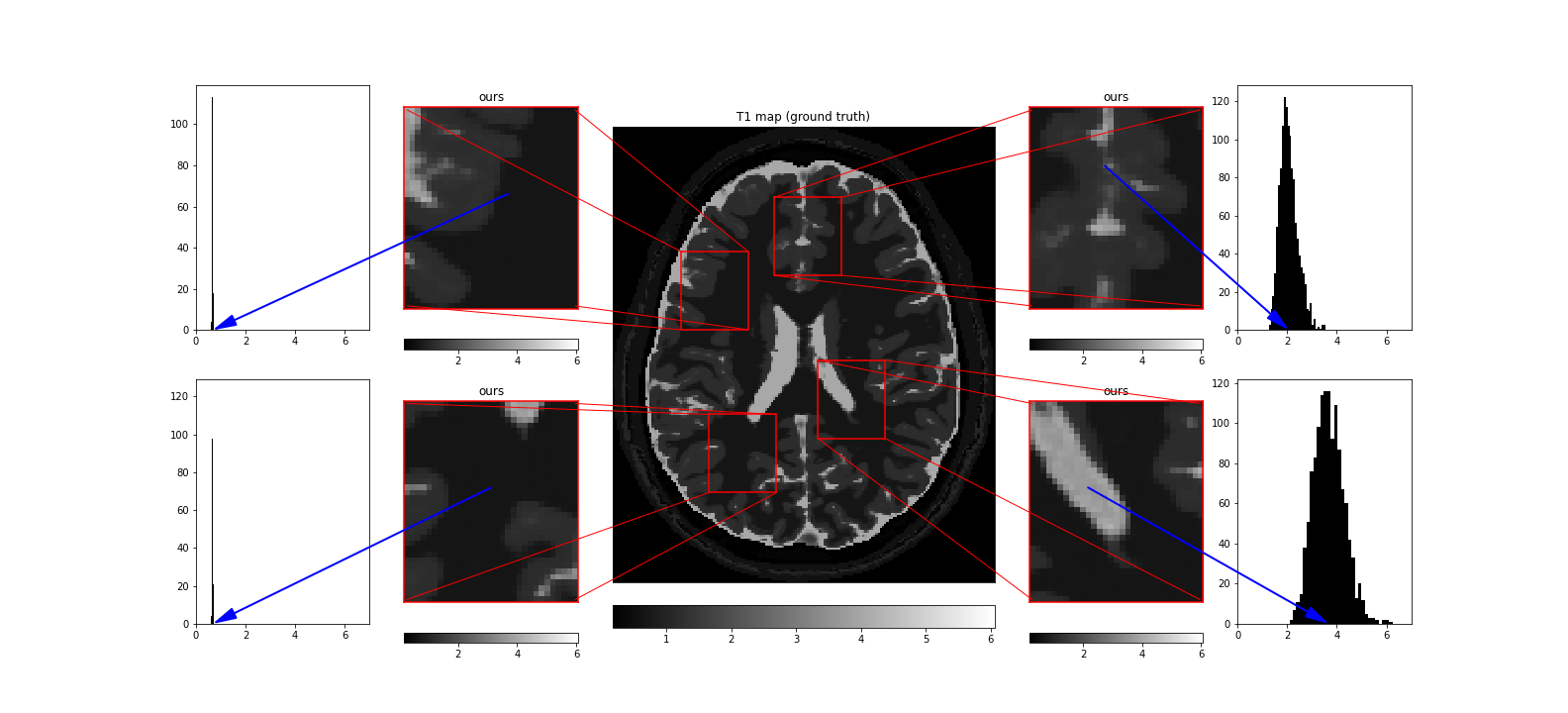
T1 parameter map (in seconds) obtained with our method (same data as in figure 1), compared to ground truth-reference. The histograms present the sampling distribution (at the pixel indicated with the blue arrow) which gives information on the uncertainty in the estimation process.
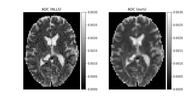
In-vivo ADC parameter map (in $$$\mathrm{mm}^2/\mathrm{s}$$$) obtained with our method (mean image over 1280 samples, after 100k optimization steps) and NLLS as reference. The acquisition was gathered with b-values 200.0, 400.0, and 800.0 $$$\mathrm{s}/\mathrm{mm}^2$$$.
DOI: https://doi.org/10.58530/2022/0373