0361

The impact and correction of inter-scan motion artefacts in variable flip angle R1 mapping at 3T and 7T

Martina F Callaghan¹, Ali Aghaeifar^1,2, Yael Balbastre^1,3, and Nadège Corbin^1,4
¹Wellcome Centre for Human Neuroimaging, UCL Queen Square Institute of Neurology, London, United Kingdom, ²MR Research Collaborations, Siemens Healthcare Limited, Frimley, United Kingdom, ³Athinoula A. Martinos Center for Biomedical Imaging, Massachusetts General Hospital and Harvard Medical School, Boston, MA, United States, ⁴Centre de Résonance Magnétique des Systèmes Biologiques, CNRS/University Bordeaux, Bordeaux, France

Synopsis

Images acquired with variable nominal flip angle (VFA) can be combined with a map of the transmit field efficiency and a signal model to estimate the longitudinal relaxation rate, R₁. However, if motion occurs between the acquisition of the VFA volumes the inherent assumptions of consistent receive field modulation and transmit field efficiency can be violated causing substantial errors in R₁. Through in vivo experiment and simulation we show that the differential receive field modulation introduces the largest amount of error. We further show that the majority of the error can be mitigated with a simple, time efficient correction.

Introduction

Images acquired with variable flip angle (VFA) can be combined with knowledge of transmit field efficiency, $$$f_{T}$$$, and a signal model to estimate the longitudinal relaxation rate, R₁. These models assume constant receive field modulation and transmit field efficiency across acquisitions. Inter-scan motion violates this assumption, even if the individual volumes are artefact-free¹. Here we quantify these errors and their reduction by a simple correction.

METHODS: R1 Computation

Assuming short TR, small $$$\alpha$$$, transmit field efficiency, $$$f_T$$$ and perfect spoiling, the gradient echo signal is:
$$I=\frac{sAf_T\alpha TRR_1}{\frac{(f_T\alpha)^2}{2}+TRR_1}$$
$$$A$$$ embeds proton density and $$$T_2^*$$$ decay, and $$$s$$$ is the receiver's sensitivity. Allowing for volume-specific transmit $$$(f_{T_1}\neq f_{T_2})$$$ and receive $$$(s_1\neq s_2)$$$ fields, R1 is estimated from two VFA volumes as²:
$$R_1=\frac{\frac{I_1f_{T_1 }\alpha_1}{2TR_1}-\frac{\Delta_{1,2}I_2 f_{T_2}\alpha_2}{2TR_2}}{\frac{\Delta_{1,2}I_2}{f_{T_2}\alpha_2}-\frac{I_1}{f_{T_1}\alpha_1}}$$

$$$\Delta_{1,2}=\frac{s_1}{s_2}$$$ is the relative receive field modulation. R₁ maps were computed with the hMRI toolbox (hmri.info) modified to accommodate this.

METHODS: Correction of receive field effects

The ratio, $$$\kappa_{1,2}$$$, of calibration images, $$$x_j$$$, with nominal flip angle $$$\alpha_c$$$, $$$TR_c$$$ and transmit efficiencies $$$f_{T_j},j\in[1,2]$$$ can be used as a proxy for the relative receive sensitivity, $$$\Delta_{1,2}$$$:

$$\kappa_{1,2}=\frac{x_1}{x_2} =\frac{s_1Af_{T_1}\alpha_cTR_cR_1}{\frac{f_{T_1}^2\alpha_c^2}{2}+TR_cR_1}. \frac{\frac{f_{T_2}^2 \alpha_c^2}{2}+TR_c R_1}{s_2Af_{T_2}\alpha_cTR_cR_1}=\frac{s_1}{s_2}.\frac{f_{T_1}f_{T_2}^2 \alpha_c^2+f_{T_1}2TR_cR_1}{f_{T_2}f_{T_1}^2\alpha_c^2+f_{T_2}2TR_cR_1} =Δ_{1,2}\frac{\partial\kappa_{1,2}}{\partial\Delta_{1,2}}$$

The correction assumes $$$\kappa_{1,2}$$$ equals the relative receive field, i.e. $$$\frac{\partial\kappa_{1,2}}{\partial\Delta_{1,2}}=1$$$. The necessary conditions are derived below.

METHODS: In vivo Experiments

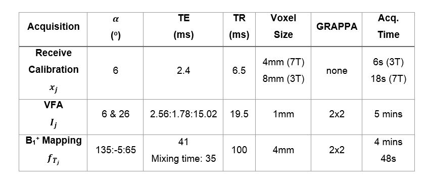
Experiments were conducted at 3T (Siemens MAGNETOM Prisma) and 7T (Siemens MAGNETOM Terra). See Table1 for key parameters. VFA data, $$$I_j,j\in[1,2]$$$, with nominal flip angle, $$$\alpha_j$$$ were acquired three times: twice in the same position and once after deliberate inter-scan movement. $$$f_T$$$ was mapped in each position³. A rapid, low resolution gradient-echo image, $$$x_j$$$, was acquired prior to each VFA volume to map the relative receive field across positions⁴. Three R₁ maps from each VFA repetition with no deliberate inter-scan motion were averaged to create a reference with respect to which error was computed. Additional R₁ maps were computed by permuting the available data. Those combined across positions were classed as motion-corrupted. Those from the same position were classed as motion-free.

METHODS: Error Analysis

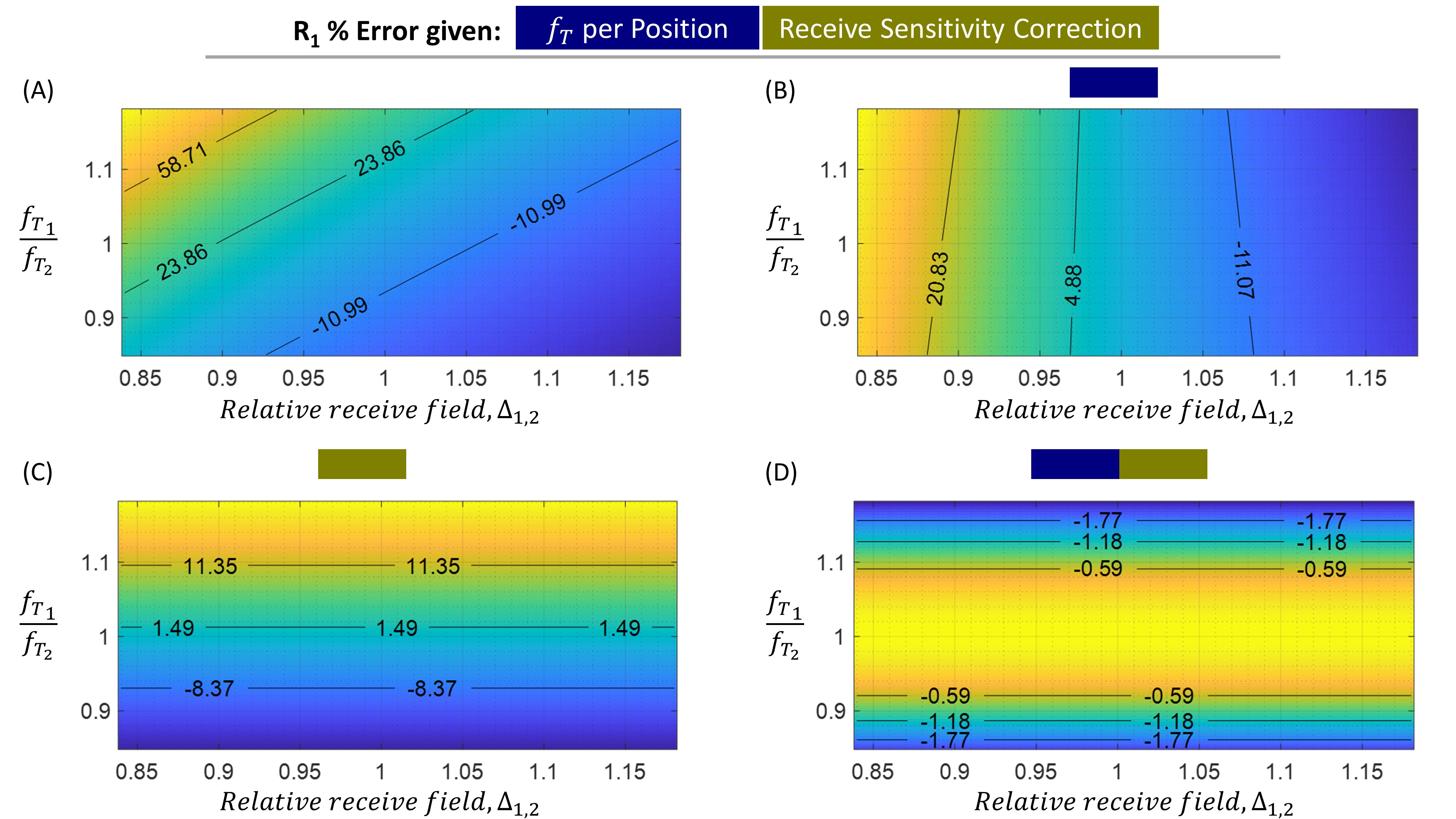
Numerically, errors were computed for $$$f_{T_1}\in[0.5,1.5], f_{T_2} =1$$$ and R₁ $$$\in[0.5,1.4]s^{-1}$$$ over the empirically observed range of relative transmit and receive fields. The median proportion of error arising from transmit or receive field changes was computed.

Numerically, and in vivo, percentage R₁ error was computed for the following cases:

Using only the first position’s B₁⁺ map, $$$f_{T_1}$$$
Incorporating calibration data to correct receive field effects
Using position-specific B₁⁺ maps, $$$f_{T_j}$$$
Combining 2 and 3.

RESULTS: Sensitivity of receive field correction

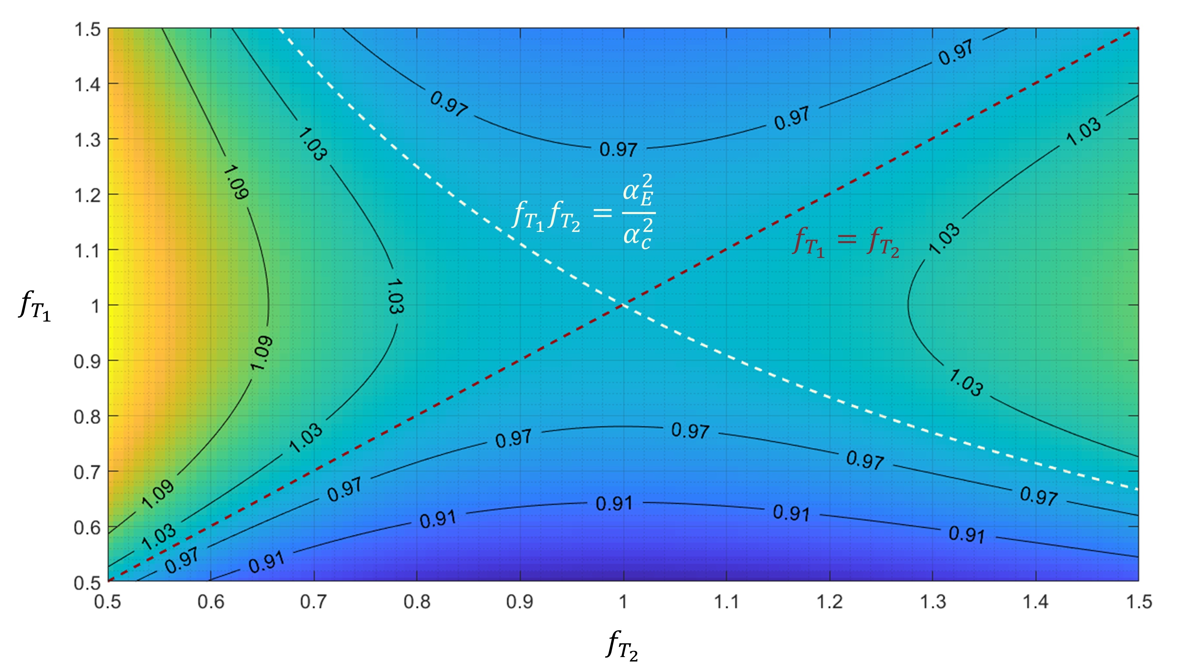
The ratio of the calibration images, $$$\kappa_{1,2}$$$, will equal the relative sensitivity, $$$\Delta_{1,2}$$$ when:

$$\frac{\partial\kappa_{1,2}}{\partial\Delta_{1,2}}=\frac{f_{T_1}f_{T_2}^2\alpha_c^2+f_{T_1}2TR_cR_1}{f_{T_2}f_{T_1}^2\alpha_c^2+f_{T_2}2TR_cR_1}=1$$

Given the Ernst angle, $$$\alpha_E=2TR_cR_1$$$, rearranging gives:

$$\frac{\alpha_E^2}{\alpha_c^2}(f_{T_2}-f_{T_1})=f_{T_1}f_{T_2}(f_{T_2 }-f_{T_1})$$

This condition is met when $$$f_{T_1}=f_{T_2}$$$, i.e. there is no change in transmit field, or when $$$f_{T_1}f_{T_2}=\frac{\alpha_E^2}{\alpha_c^2}$$$. These conditions are highlighted in Fig.1 which shows $$$\frac{\partial\kappa_{1,2}}{\partial\Delta_{1,2}}$$$ as a function of $$$f_{T_j}$$$ for R₁=0.84s^-1. Deviation of $$$\frac{\partial\kappa_{1,2}}{\partial\Delta_{1,2}}$$$ from 1 is <3% for a broad range of values centred on both acquisitions being at the Ernst angle.

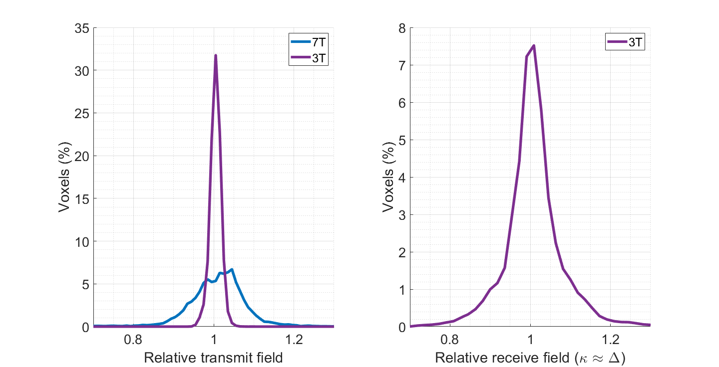
RESULTS: Relative fields after inter-scan motion: Fig.2

At 3T the relative transmit efficiency ranged from 0.97 to 1.04. The relative receive field (measured via $$$\kappa_{1,2}$$$) ranged from 0.84 to 1.18. At 7T the relative transmit efficiency ranged from 0.85 to 1.18 under comparable motion conditions.

RESULTS: Numerical R1 Error

Uncorrected, inter-scan motion caused errors up to 136%. Over the 4D parameter space investigated, a median of 29% of the error was caused by transmit field effects and 71% by receive field effects. Fig.3 shows a plane of this error as the relative transmit and receive fields change. Position-specific $$$f_T$$$ offers only partial correction (Fig.3B). Larger error reduction arises from receive field correction (Fig.3C). Combining both (Fig.3D) shows receive field effects are removed but transmit sensitivity remains (when $$$\frac{\partial\kappa}{\partial\Delta_{1,2}}\neq1$$$).

RESULTS: Empirical R1 Error

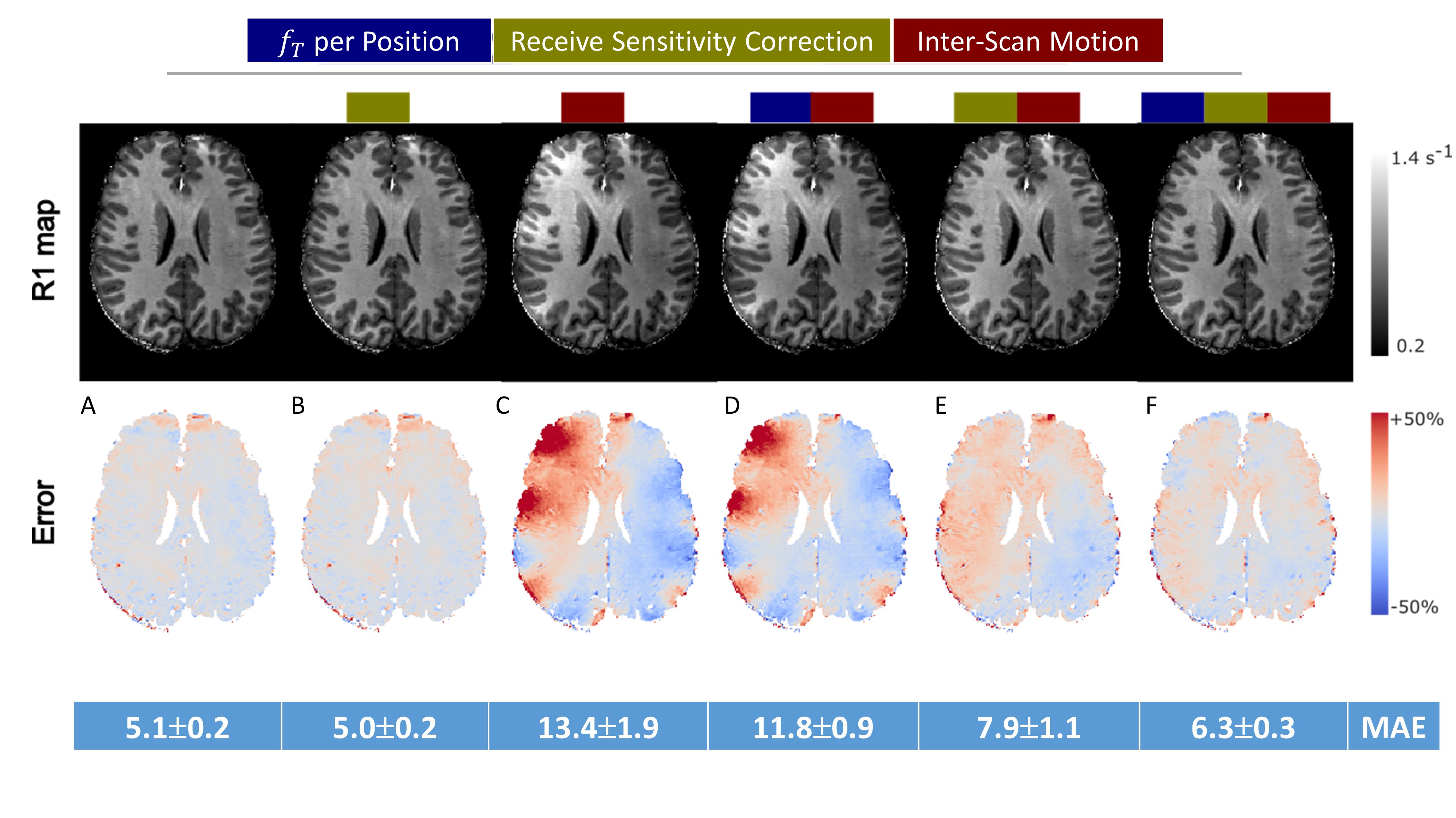
In the absence of motion, the proposed receive field correction did not introduce error (Fig.4A v’s Fig.4B). Inter-scan motion introduced substantial error (Fig.4C), which was partially reduced by per-position transmit efficiencies (Fig.4D), but more so by receive field correction (Fig.4E). The largest error reduction was obtained by combining corrections (Fig.4F).

DISCUSSION

Motion-induced changes in transmit fields are much larger at 7T than 3T (Fig.2), and on a par with receive field changes, which could only be estimated at 3T due to the confounding effect of transmit field changes at 7T. Experiment and simulation consistently showed that receive field changes cause much larger R₁ errors (Figs.3,4).

The time consuming nature of accurate B₁⁺ mapping makes routine repetition infeasible. However, the calibration data facilitating receive field correction are rapid (<18s) and a small fraction of the VFA acquisition time. This correction does not introduce error in the absence of motion (Fig.4B) yet achieves substantial error reduction in the presence of motion (Fig.4E). Therefore it is always recommended for VFA-based R₁ mapping.

Examining the conditions at which the correction will have the target sensitivity to receive field changes led to the condition $$$f_{T_1}f_{T_2}=\frac{\alpha_E^2}{\alpha_c^2}$$$. Consequently, the calibration data should be acquired at the Ernst angle of the mean expected R₁. This will maximise SNR and robustness to transmit field changes (Fig.1). At 3T receive field correction is expected to reduce errors to <1% (Fig.3).

CONCLUSION

Inter-scan motion causes substantial R1 error, predominantly caused by receive field changes. A simple correction scheme has potential transmit sensitivity but is shown to remove the majority of error, particularly at 3T and when using the Ernst angle.

Acknowledgements

This research was supported by the MRC and Spinal Research Charity through the ERA-NET Neuron joint call (MR/R000050/1). The Wellcome Centre for Human Neuroimaging is supported by core funding from the Wellcome [203147/Z/16/Z].

References

1. Papp, D., Callaghan, M. F., Meyer, H., Buckley, C. & Weiskopf, N. Correction of inter-scan motion artifacts in quantitative R1 mapping by accounting for receive coil sensitivity effects. Magn. Reson. Med. 76, 1478–1485 (2016).

2. Helms, G., Dathe, H. & Dechent, P. Quantitative FLASH MRI at 3T using a rational approximation of the Ernst equation. Magn. Reson. Med. 59, 667–72 (2008).

3. Lutti, A. et al. Robust and Fast Whole Brain Mapping of the RF Transmit Field B1 at 7T. PLoS One 7, e32379 (2012).

4. Balbastre, Y. et al. Correcting inter-scan motion artefacts in quantitative R1 mapping at 7T. 1–11 (2021). at <http://arxiv.org/abs/2108.10943>

Figures

Figure 1: δκ/δΔ. Sensitivity of the receive field correction to transmit field efficiency at each position for an R₁ of 0.84s^-1. When there is no motion-induced change in the transmit field (red line) the correction will remove the receive field error fully. This will also occur when the product of the efficiencies equals the square of the ratio of the Ernst angle, α_E, to the calibration data flip angle, α_C. When this condition is met the calibration images will again have matching signal intensities, but on either side of the Ernst angle.

Figure 2: Histograms of relative transmit field after inter-scan motion at 3T and 7T (left). At 3T, the ratio of the calibration data, κ_1,2, was used as a proxy for the relative receive field (right) under the assumption of static transmit field, a reasonable assumption at 3T. The range spanned by these distributions are reported as (median - 2*inter-quartile-range) to (median + 2*inter-quartile-range) to capture 99% of voxels.

Figure 3: Numerical analysis of the error in R₁ caused by inter-scan motion with R₁ = 0.84s^-1 and f_T2 = 1. The relative transmit field efficiency, f_T1/f_T2, ranged from 0.85 to 1.18 (7T experiment) and the relative receive field, Δ_1,2, ranged from 0.84 to 1.18 (3T experiment). Sequence settings (flip angles and TRs) matched those used in the experiments (Table1). Contours indicate percentage error. Note the calibration flip angle equals the Ernst angle in this example.

Figure 4: 7T R₁ maps (top) and error (bottom) with respect to the reference. No motion without (A) and with (B) receive sensitivity correction. Inter-scan motion with no correction (C), per-position transmit fields (D), receive field correction (E) or both (F). MAE: mean absolute error over voxels with respect to the reference summarised by the mean and standard deviation over R₁ maps per condition. The net (root mean square across orthogonal axes) translation and rotation of the inter-scan motion case were 4.6 mm and 11.2 degrees respectively.

Table 1: Key sequence parameters. The VFA and receive field acquisitions were spoiled gradient echoes. The B₁⁺ mapping was based on the acquisition of 15 pairs of spin and stimulated echoes, together with B₀ mapping data to unwarp spatial distortions.

Proc. Intl. Soc. Mag. Reson. Med. 30 (2022)

0361

DOI: https://doi.org/10.58530/2022/0361