0340
Learning Time-Adaptive Data-Driven Sampling Pattern for Accelerated 3D Myocardial Perfusion Imaging
Valery Vishnevskiy1, Tobias Hoh1, and Sebastian Kozerke1
1University and ETH Zurich, Zurich, Switzerland
1University and ETH Zurich, Zurich, Switzerland
Synopsis
We investigated potential benefits of optimizing accelerated 3D myocardial perfusion MRI by time-adaptive data-driven k-t Cartesian sampling during the scan. To this end, the sampling mask for each following acquisition window is inferred by a neural network on the fly using the acquired history of MR signal projections. It is demonstrated that time-adaptive data-driven sampling reduces reconstruction errors by 25% along with a reduction of signal underestimation during the contrast bolus passage when compared to a predefined fixed sampling pattern.
Introduction
Dynamic 3D+t perfusion MRI requires highly accelerated data sampling due to a short acquisition window during the cardiac cycle. Variable density (VD) sampling strategies, where low frequencies are sampled more densely, allow to improve compressed sensing (CS) reconstruction accuracy compared to uniform undersampling1,2. Undersampling mask optimization for spatial encoding was researched in the context of model- and data-based image reconstruction3,4. However, in the case of dynamic imaging, CS reconstruction tends to oversmooth and, therefore, underestimate extreme signal characteristics, which are often useful for clinical diagnosis5. In the present work we investigated the feasibility of conditioning the k-t sampling pattern on the observed data to account for image intensity variation due to contrast agent arrival with time (Figure 1). Namely, we propose to generate sampling masks on the fly using a neural network that is fed with time-dependent object projections (DC) derived from the k-space center.Methods
Given 3D+t perfusion imaging data $$$\rho$$$ of size $$$n_x\times n_y\times n_z\times n_t$$$, the undersampled k-space is modeled as $$$\mathbf{k}=\mathbf{m} \odot \mathbf{F}\rho$$$, where $$$\mathbf{F}$$$ is Cartesian Fourier transform, $$$\mathbf{m}$$$ a binary sampling mask of size $$$n_y\times n_z \times n_t$$$ generated from a probability map $$$\mathbf{p}$$$ as realizations of Bernoulli random variables: $$$m_i=[\mathcal{U}(0,1) < p_i]\sim\mathcal{B}(p_i)$$$, where $$$i$$$ are the sample indices. We parametrize the sampling probability map $$$\mathbf{p}$$$ with logits: $$$p_i=(1+\exp(-q_i))^{-1}=\sigma(q_i)$$$. While logits are parametrized by the exponentiated quadratic form $$$q_{t,i}=(\mathbf{\kappa}_i^T\mathbf{\Lambda}_t\mathbf{\kappa}_i)^{\gamma_t}+s_t$$$, where $$$\mathbf{\kappa}_i$$$ is the k-space coordinate, $$$t$$$ is the temporal index and $$$\mathbf{\Lambda}_t$$$ is a positive-definite matrix. The parametrization coefficients are predicted by a fully connected (FC) network with weights $$$\phi$$$, based on $$$T_s$$$ preceding DC values: $$$\text{FC}_\phi: \{DC(t - T_s),\dots,DC(t - 1)\}\rightarrow\{\mathbf{\Lambda}_t,s_t,\gamma_t\}$$$. The FC network consists of 4 layers (16, 32, 16, 5 neurons) with ReLU activations (except for the output layer). The positive-definiteness of $$$\mathbf{\Lambda}_t$$$ is guaranteed by predicting a Cholesky factor matrix with nonnegative diagonal. The sampling budget constraints (fixed number of samples per acquisition window) are enforced by non-linear least squares projections (Figure 2). As a shorthand for aforementioned steps, we note that masks are generated by the SamplingNet: $$$\mathbf{m}\sim\text{SampleNet}_\phi$$$.Learning-based image reconstruction $$$\hat{\rho}=\mathcal{V}_\theta(\mathbf{k})$$$ can be achieved with a model-informed neural network6,8 $$$\mathcal{V}_\theta$$$ with weights $$$\theta$$$. In order to increase the generalization ability, we used an ADMM-Net7 inspired architecture by unrolling 10 iterations of the vectorial total variation8 regularized reconstruction. Since the convolutional filters were fixed, the network has only 50 trainable weights (1 gradient descent step length, 1 penalty parameter, 3 shrinkage coefficients per layer). Given a set of training images $$$\mathcal{T}$$$ we jointly optimize the reconstruction network and SamplingNet using 104 alternating iterations of the Adam algorithm:
$$\min_{\phi}\; \mathbb{E}_{\mathbf{m}\sim\text{SamplingNet}_\phi}\; \min_\theta \mathbb{E}_{\rho\sim\mathcal{T}}\; \|\mathcal{V}_\theta(\mathbf{m}\odot\mathbf{F}\rho)-\rho\|_1.$$
Loss gradient values w.r.t. reconstruction network weights $$$\theta$$$ are calculated via backpropagation, while gradients w.r.t. SamplingNet weights $$$\phi$$$ are calculated using the RELAX algorithm10,11 with the critic network $$$\mathcal{C}_\tau(\mathbf{l}, \mathbf{F}\rho)=\mathcal{V}_\theta(\sigma(\mathbf{l}\cdot\exp(\tau))\odot\mathbf{F}\rho)$$$, where $$$\mathbf{l}$$$ are the corresponding mask logits and relaxation parameter $$$\tau=-3$$$.
Training perfusion imaging data were acquired from 5 healthy volunteers upon written informed consent on a 1.5 T Philips MR system (Philips Healthcare, The Netherlands) using a 5-element cardiac coil array with 10x undersampled VD-sampling masks. Imaging parameters were: TR/TE = 2.0/1.0 ms, spatial resolution: 2.5x2.5x10 mm3, FA:15°, acquisition window: 240 ms, and a saturation delay: 135 ms. Contrast agent (Gadovist, Germany) bolus injections of 0.075 mmol/kg b.w. at 4 ml/s were performed during rest. Images were reconstructed using the MI-LLR algorithm12.
During time-adaptive data-driven sampling a single uniform coil sensitivity map was assumed, allowing a more challenging reconstruction scenario with the same acceleration factor $$$r=10$$$ not relying on additional coil encoding. The SamplingNet trained using data from 4 volunteers. During the test, sampling masks were generated by the SamplingNet and reconstructed using the model-based locally low-rank (LLR) algorithm13 with optimal regularization value and patch size of 163 voxels.
Results
Predicted sampling masks and probabilities with LLR reconstructions are presented in Figure 3. The SamplingNet tends to oversample low frequency k-space regions during time frames corresponding to contrast agent arrival. The analysis presented in Figure 4 shows that low and high frequency sampling is alternated, while high frequency sampling is preferred for frames with (i)lower image intensity and (ii)lower intensity variation. The comparison of reconstructions in Figure 5a indicates image nRMSE improvement of 25% in the cardiac region. Moreover, signal intensity curves in Figure 5b show that the proposed optimization allows to reduce signal underestimation.Discussion
A learning based time-adaptive approach to optimize undersampling patterns on the fly based on object projections (DC) has been realized. The resulting signal curves, averaged over cardiac segments, show reduced signal underestimation, potentially leading to improved myocardial perfusion parameter fitting. The masks inferred by the SamplingNet can be intuitively interpreted and allow a favorable balance between random sampling incoherence and dependence on the observed signal dynamics. The sampling strategy can be optimized to improve reconstruction in a specific cardiac region.Conclusion
We have demonstrated that time-adaptive data-driven Cartesian sampling allows to improve reconstruction quality as compared to a standard time-invariant undersampling for accelerated 3D myocardial perfusion imaging. The method uses limited information (preceding DC values) to infer sampling masks, which allows an efficient real-time deployment on MR scanners towards self-driving and self-learning MR imaging.Acknowledgements
Funding of the Swiss National Science Foundation, grant 325230_197702, is gratefully acknowledged.References
1. Schmidt J, Santelli C, and Kozerke S. Optimized k-t Sampling for Combined Parallel Imaging and Compressed Sensing Reconstruction. Proc. Intl. Soc. Mag. Reson. Med. 22, 2014.2. Knoll F, Hammernik K, et al. Assessment of the generalization of learned image reconstruction and the potential for transfer learning. Magnetic resonance in medicine, 2018.
3. Bahadir C, Dalca A, Sabuncu M. Learning-based optimization of the under-sampling pattern in MRI. InInternational Conference on Information Processing in Medical Imaging 2019 Jun 2 (pp. 780-792). Springer, Cham.
4. Seeger M, Nickisch H, Pohmann R, Schölkopf B. Optimization of k‐space trajectories for compressed sensing by Bayesian experimental design. Magnetic Resonance in Medicine: An Official Journal of the International Society for Magnetic Resonance in Medicine. 2010 Jan;63(1):116-26.
5. Vishnevskiy V, Walheim J, Kozerke S. Deep variational network for rapid 4D flow MRI reconstruction. Nature Machine Intelligence. 2020 Apr;2(4):228-35.
6. Hammernik K, Klatzer T, Kobler E, Recht MP, Sodickson DK, Pock T, Knoll F. Learning a variational network for reconstruction of accelerated MRI data. Magnetic resonance in medicine. 2018 Jun;79(6):3055-71.
7. Yang Y, Sun J, Li H, Xu Z. Deep ADMM-Net for compressive sensing MRI. In Proceedings of the 30th international conference on neural information processing systems 2016 Dec 5 (pp. 10-18).
8. Blomgren P, Chan TF. Color TV: total variation methods for restoration of vector-valued images. IEEE transactions on image processing. 1998 Mar.
9. Diederik P Kingma and Jimmy Ba. Adam: A method for stochastic opti-
mization. arXiv preprint:1412.6980, 2014.
10. Grathwohl W, Choi D, Wu Y, Roeder G, Duvenaud D. Backpropagation through the void: Optimizing control variates for black-box gradient estimation. arXiv preprint arXiv:1711.00123. 2017 Oct 31.
11. Gadetsky A, Struminsky K, Robinson C, Quadrianto N, Vetrov D. Low-variance black-box gradient estimates for the plackett-luce distribution. InProceedings of the AAAI Conference on Artificial Intelligence 2020 Apr 3 (Vol. 34, No. 06, pp. 10126-10135).
12. Tobias Hoh, Valery Vishnevskiy, Maximilian Fuetterer, Sebastian Kozerke. Free-Breathing Motion-Informed Quantitative 3D Myocardial Perfusion Imaging. Proc. ISMRM 2021.
13. Zhang T, Pauly JM, Levesque IR. Accelerating parameter mapping with a locally low rank constraint. Magnetic resonance in medicine. 2015 Feb;73(2):655-61.
Figures
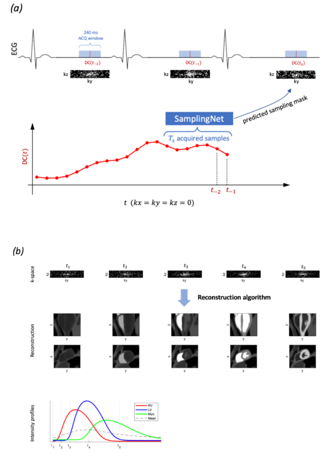
Figure 1: (a) Overview of dynamic, cardiac-triggered 3D perfusion imaging with time-adaptive undersampling guided by the DC-signals recorded in preceding $$$T_s$$$ intervals, which serve as input to the SamplingNet which predicts an optimal sampling mask for the next acquisition interval at $$$t_0$$$. (b) Reconstruction of 3D+time imaging data collected with time-adaptive sampling. The contrast agent dynamics determines temporal image contrast variations as exemplified by time-intensity profiles of the right ventricle (RV), left ventricle (LV) and myocardium (Myo).
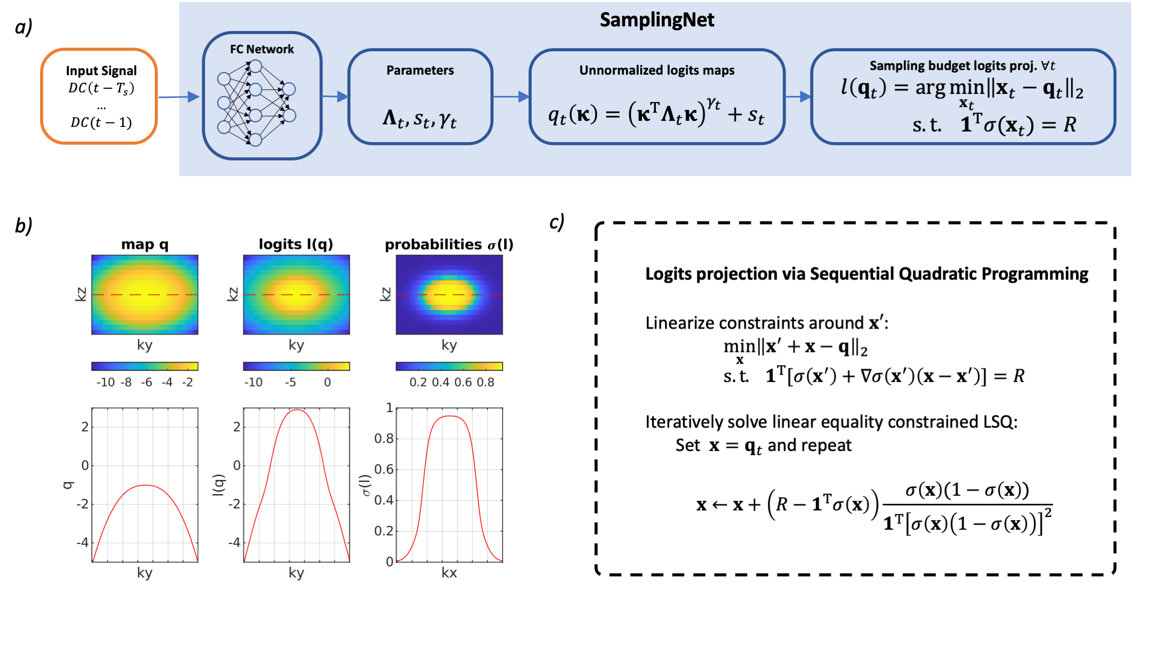
Figure 2: Sampling network architecture. (a) $$$T_s$$$ preceding DC- components are passed to a fully connected (FC) neural network that predicts logit parametrization and guarantees sampling constraints by nonlinear projection, where $$$R=n_y n_z /r$$$ is the sampling budget per time frame. (b) Illustration of the logits projection step. Note that $$$l(\mathbf{q})$$$ is a nonlinear operation.(c) Logits projection via sequential quadratic programming. In practice, the algorithm converges in 3-7 iterations, and is differentiable w.r.t. input $$$q$$$.
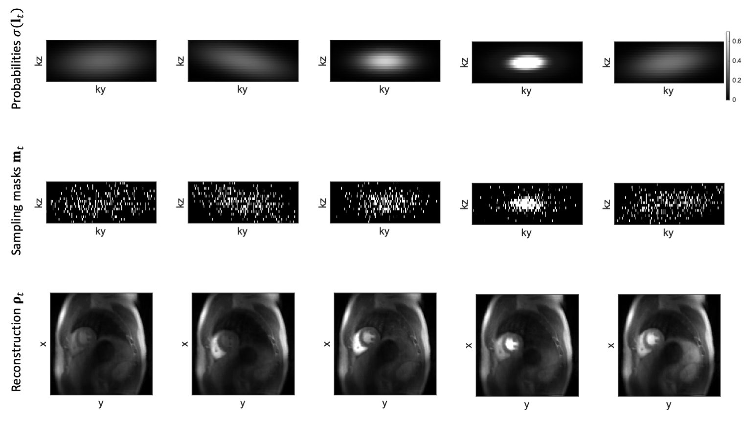
Figure 3: Predicted probability maps with corresponding sampling masks and LLR reconstructions for an acceleration factor of 10. Note the sampling mask density variation as a function of contrast agent passage.
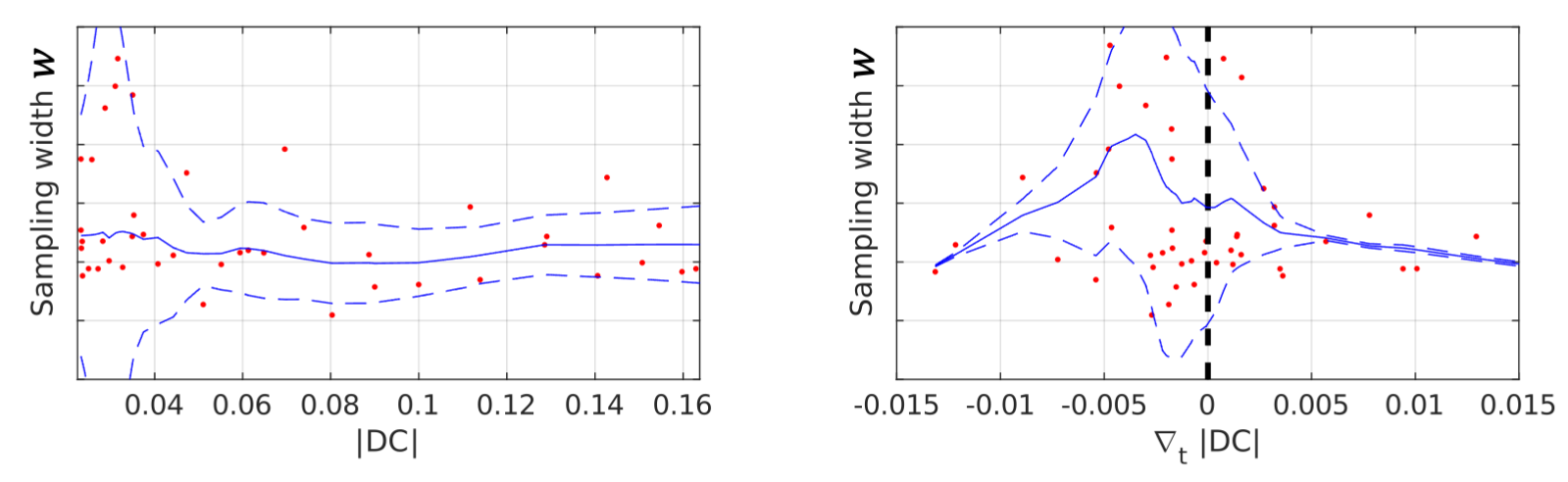
Figure 4: Sampling density at acquired dynamics vs. DC magnitude (left) and its temporal derivative (right). The sampling width $$$w=\sum_\kappa |\kappa|\sigma(l(\mathbf{\kappa}))$$$. Low values of $$$w$$$ indicate the k-space center is oversampling, high values of $$$w$$$ indicate that more of the high frequencies are sampled. The figure on the right suggests that sampling high frequencies is the most efficient strategy for dynamics with lower signal variation ($$$\nabla_t|DC|\approx0$$$). Smoothing (blue line ±std) is conducted with local polynomial regression.
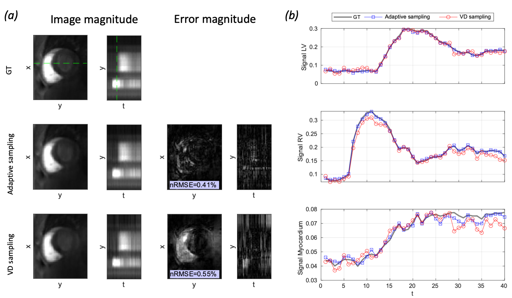
Figure 5: 10x accelerated 3D+t perfusion acquisition with time-adaptive, data-driven sampling. (a) Registered LLR reconstruction and error analysis with (i) the proposed adaptive and (ii) standard variable density (VD) masks. Temporal y-t profile locations are indicated by the green dashed line. (b) Mean signal intensity over left and right ventricles and myocardium for the reconstructions versus ground truth (GT). Note the signal underestimation for VD sampling masks, which is not seen with adaptive sampling
DOI: https://doi.org/10.58530/2022/0340