0298
Using data-driven Markov chains for MRI reconstruction with Joint Uncertainty Estimation1University Medical Center Göttingen, Göttingen, Germany, 2Institute of Medical Engineering, Graz, Austria, 3German Centre for Cardiovascular Research (DZHK), Partner Site Göttingen, Göttingen, Germany, 4Cluster of Excellence "Multiscale Bioimaging: from Molecular Machines to Networks of Excitable Cells'' (MBExC), University of Göttingen, Göttingen, Germany
Synopsis
This works explores the use of data-driven Markov chains that are constructed from generative models for Bayesian MRI reconstruction, where the generative models utilize prior knowledge learned from an existing image database. Given the measured k-space, samples are then drawn from the posterior using Markov chain Monte Carlo (MCMC) method. In addition to the maximum a posteriori (MAP) estimate for the image which is obtained with conventional methods, also a minimum mean square error (MMSE) estimate and uncertainty maps can be computed from these samples.
Introduction
We introduce a framework which enables efficient sampling from complex probability distributions for MRI reconstruction. Different from conventional deep learning-based MRI reconstruction techniques, the reconstruction is achieved with data-driven Markov chains that are constructed with generative models. Given the measured k-space, samples are drawn from the posterior term using Markov chain Monte Carlo (MCMC) method. In addition to the maximum a posteriori (MAP) estimate for the image which is obtained with conventional methods, also a minimum mean square error (MMSE) estimate and uncertainty maps can be computed from these samples. The generative models utilize the prior knowledge learned from an image database. These models are independent from the forward operator that is used to model the k-space measurement. This provides flexibility because the method can be applied to k-space acquired with a different sampling scheme using the same pre-trained models.Theory
With samples drawn from the posterior term $$$p(\mathbf{x}|\mathbf{y})$$$ with data-driven Markov chains1$$\tilde{p}(\mathbf{x}_{i} \mid \mathbf{x}_{i+1}) \approx \mathcal{N}(\mathbf{x}_{i} ; (1-\lambda\tau_{i+1}\mathcal{A}^{H}\mathcal{A})\mathbf{\mu}_{\mathbf{\theta}}(\mathbf{x}_{i+1}, i+1)+\lambda\tau_{i+1}(\mathcal{A}^{H}\mathbf{y}_0-\mathcal{A}^{H}\mathcal{A}\mathbf{z}_{\sigma_i}), \tau_{i+1}^{2} \mathbf{I}), \quad (1)$$
the MMSE reconstruction $$$\mathbf{x}_\mathrm{MMSE}$$$ and the uncertainty map are obtained. The sampling is performed with Langevin Dynamics at each intermediate distribution.
Methods
To construct learned Markov chains $$$\tilde{p}(\mathbf{x}_{i} \mid \mathbf{x}_{i+1})$$$, we trained two types of score networks2 $$$\mathbf{\mu}_{\mathbf{\theta}}(\mathbf{x}_{i+1}, i+1)$$$. One is conditional on discrete noise scales ($$$\mathtt{NET}_1$$$), the other is conditional on continuous noise scales ($$$\mathtt{NET}_2$$$). Following experiments are performed to investigate the proposed algorithm in Figure 1(c).(A): Single coil unfolding. The single channel k-space is simulated out of multi-channel k-space data and the odd lines in k-space are retained. We redo the experiment with the object shifted to the bottom.
(B): More noise scales. We reconstructed the image from the undersampled k-space with two score networks, respectively, that are conditional on different number of noise scales.
(C): Burn-in phase. We spawned multiple chains at a certain noise scale when drawing samples, as illustrated in Figure 1(b). For instance, let ($$$\mathbf{x}_\mathrm{MMSE}, 60$$$) denote the $$$\mathbf{x}_\mathrm{MMSE}$$$ that is computed with 10 samples drawn from $$$p(\mathbf{x}|\mathbf{y})$$$ by spawning 10 chains at the 60$$$^{th}$$$ noise scale. Changing the spawning point, we got different sets of samples that are from chains of different length.
(D): Benchmark. The fastMRI dataset was used to evaluate the performance of the proposed method. The undersampling pattern for each slice is randomly generated in all retrospective experiments.
Results and Discussions
(A): Since there is a lack of spatial information from coil sensitivities, folding artifacts still exist in $$$\mathbf{x}_\mathrm{MMSE}$$$ as shown in Figure 2, even when reconstructed with the learned Markov chains. As only odd lines are acquired, all images in which the superposition of points $$$\mathrm{P}_{l}$$$ and $$$\mathrm{P}_{l+2/n}$$$ equals to the points $$$\mathrm{P}_r$$$ in ground truth are solutions to $$$\mathbf{y}=\mathcal{A}\mathbf{x} +\epsilon$$$ with the same error. As expected, without parallel imaging, the uncertainty caused by the undersampling leads to huge error. The shift of the object increases the symmetry and then leads to even bigger errors as the learned Markov chains used images which were not shifted.(B): Curves of PSNRs and SSIMs over iterations are plotted in Figure 3(a) and (b). The PSNR and the SSIM of $$$\mathbf{x}_\mathrm{MMSE}$$$ are 36.06dB, 0.9175 ($$$\mathtt{NET}_1$$$) and 37.24dB, 0.9381 ($$$\mathtt{NET}_2$$$). The variance of the samples that are drawn with $$$\mathtt{NET}_2$$$ is less than those drawn with $$$\mathtt{NET}_1$$$, which means that we are more confident about the reconstuction using $$$\mathtt{NET}_2$$$. When we zoom into the region of more complicated structures, the boundaries between white matter and gray matter are more distinct in the image recovered with $$$\mathtt{NET}_2$$$ and the details are more obvious, as shown in Figure 3(c).
(C): The two sets of $$$\mathbf{x}_\mathrm{MMSE}$$$ are presented in Figure 4. In Figure 4(a), the earlier we spawn chains, the closer the $$$\mathbf{x}_\mathrm{MMSE}$$$ gets to the truth. Especially, when we zoom into the region of complicated structures (indicated by the red rectangle), the longer chains make fewer mistakes. However, give more k-space data points, the longer chains do not cause a huge visual difference in the $$$\mathbf{x}_\mathrm{MMSE}$$$s as shown in Figure 4(b), even though there is a slight increase in PSNR and SSIM. Although fewer data points means more uncertainties, long chains permit more sufficient exploration of the solution space.
(D): $$$\ell_1$$$-ESPIRiT denotes the reconstruction with the $$$\mathtt{pics}$$$ command of the BART3 toolbox using $$$\ell_1$$$-wavelet regularization (0.01), which mostly recovers general structures while smoothing out some details. In $$$\mathbf{x}_\mathrm{MMSE}$$$, the majority of details are recovered, and the texture is almost identical to the ground truth, although some microscopic structures are still missing. The metrics of 3 subjects are averaged over slices of each subject (Figure 4b).
Conclusion
The proposed reconstruction method combines concepts from machine learning, Bayesian inference, and image reconstruction. In the setting of Bayesian inference, the image reconstruction is realized by drawing samples from the posterior p(x|y) using data driven Markov chains. Different from conventional methods that only provide the MAP estimate, Markov chains fully explore the posterior distribution and can be used to obtain the MMSE estimate and uncertainty estimation.Acknowledgements
We acknowledge funding by the "Niedersächsisches Vorab" funding line of the Volkswagen Foundation.References
[1] Sohl-Dickstein, Jascha, et al. "Deep unsupervised learning using nonequilibrium thermodynamics." International Conference on Machine Learning. PMLR, 2015.APA
[2] Song, Yang, and Stefano Ermon. "Generative modeling by estimating gradients of the data distribution." arXiv preprint arXiv:1907.05600 (2019).
[3] Uecker, Martin, et al. mrirecon/bart: version 0.6.00, July 2020. NIH Grant U24EB029240-01.
Figures
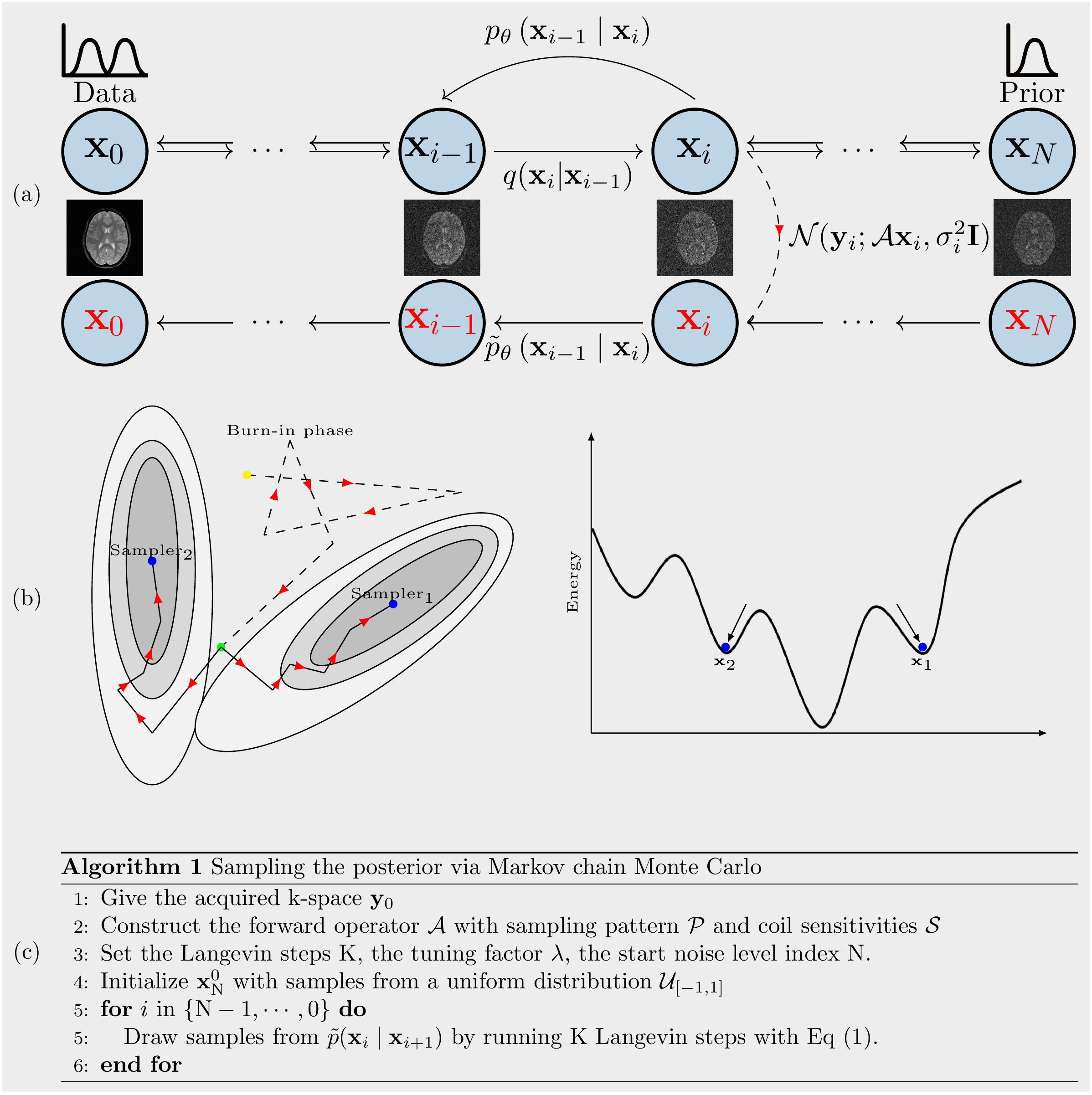
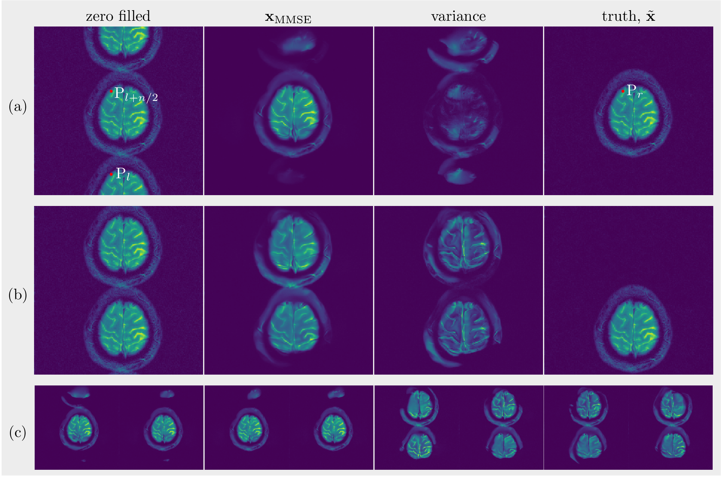
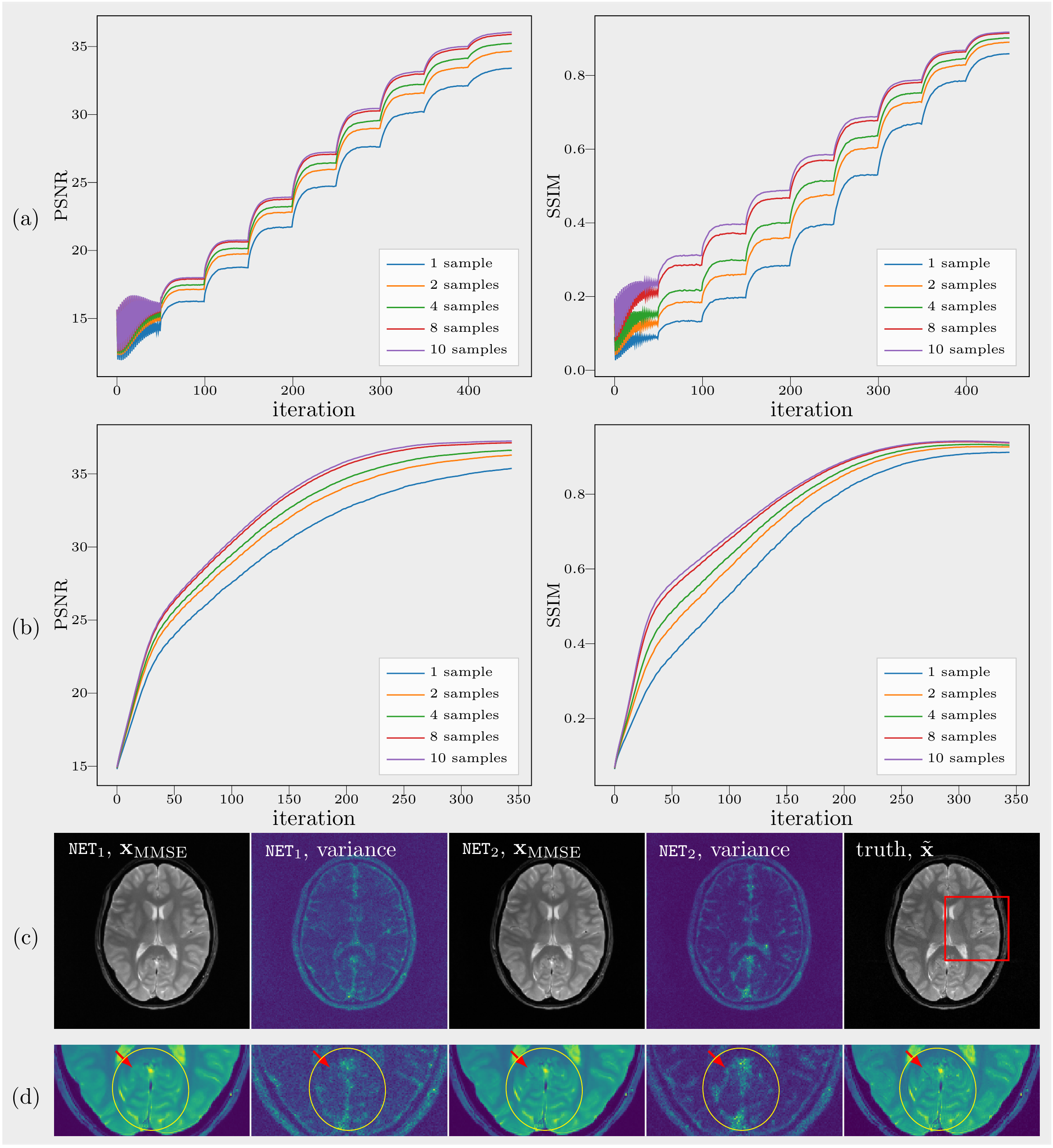
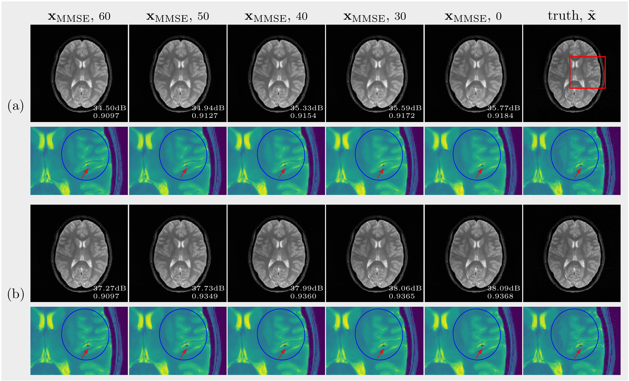
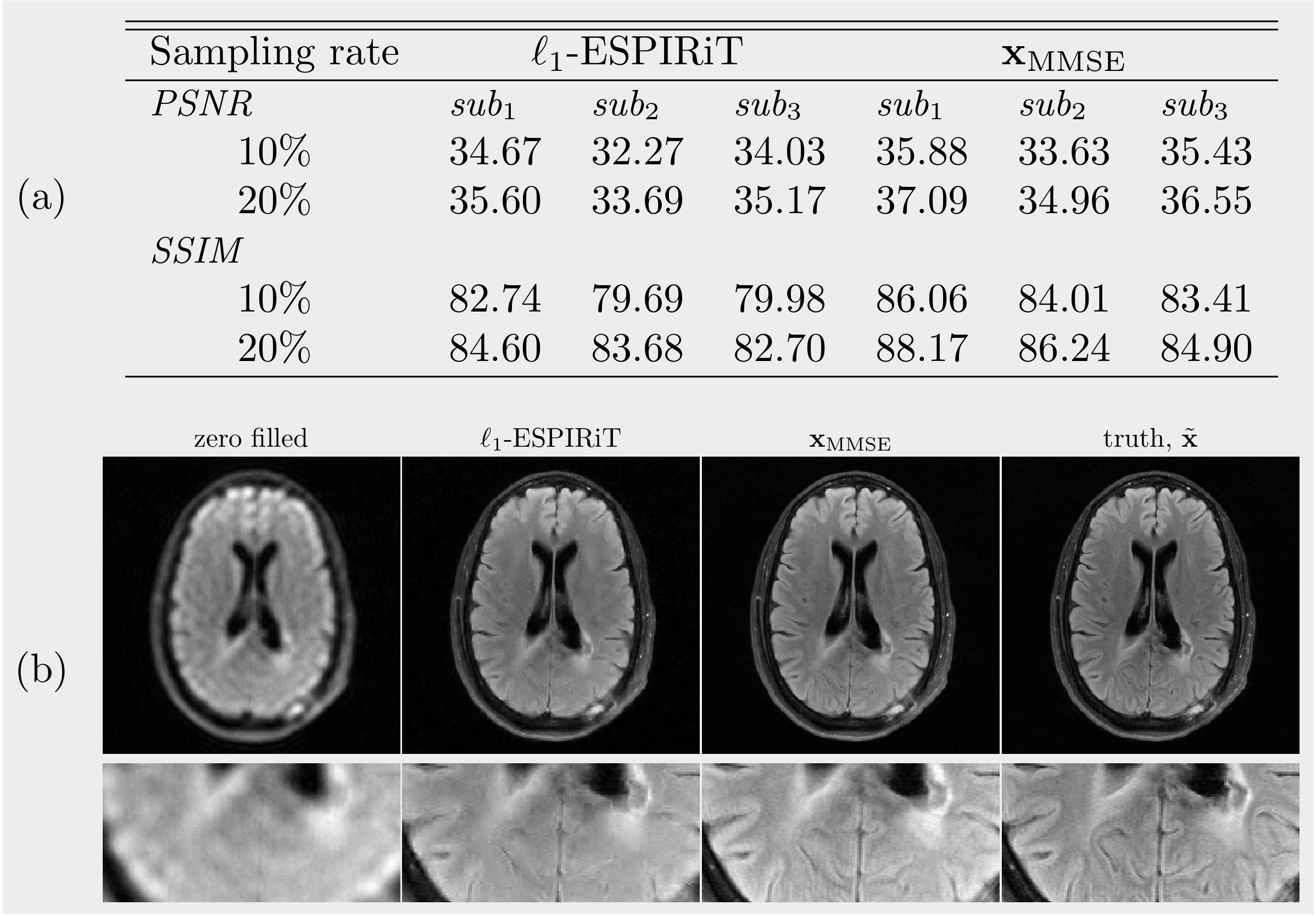
Figure 5: Performance on the open fastMRI dataset. (a) Average PSNR (dB) and SSIM(%) for 3 test subjects. (b) The high resolution image (320$$$\times$$$320) reconstructed with the k-space data of a 10-fold accelerated acquisition.