0247
Learning compact latent representations of signal evolution for improved shuffling reconstruction
Yamin Arefeen1, Junshen Xu1, Molin Zhang1, Jacob White1, Berkin Bilgic2,3, and Elfar Adalsteinsson1,4,5
1Massachusetts Institute of Technology, Cambridge, MA, United States, 2Athinoula A. Martinos Center for Biomedical Imaging, Charlestown, MA, United States, 3Department of Radiology, Harvard Medical School, Boston, MA, United States, 4Harvard-MIT Health Sciences and Technology, Cambridge, MA, United States, 5Institute for Medical Engineering and Science, Cambridge, MA, United States
1Massachusetts Institute of Technology, Cambridge, MA, United States, 2Athinoula A. Martinos Center for Biomedical Imaging, Charlestown, MA, United States, 3Department of Radiology, Harvard Medical School, Boston, MA, United States, 4Harvard-MIT Health Sciences and Technology, Cambridge, MA, United States, 5Institute for Medical Engineering and Science, Cambridge, MA, United States
Synopsis
Applying linear subspace constraints in the shuffling forward model enables reconstruction of signal dynamics through reduced degrees of freedom. Other techniques train auto-encoders to learn latent representations of signal evolution to apply as regularization. This work inserts the decoder portion of an auto-encoder directly into the shuffling forward model to reduce degrees of freedom in comparison to linear techniques. We show that auto-encoders represent fast-spin-echo signal evolution with 1 latent variable, in comparison to 3-4 linear coefficients. Then, the reduced degrees of freedom enabled by the decoder improves reconstruction results in comparison to linear constraints in simulation and in-vivo experiments.
Introduction
Linear constraints1-3 enable reconstruction of signal dynamics for improved image quality1,4,5 and quantitative parameter mapping6-9 by inserting subspaces, generated with singular-value-decompositions on dictionaries of simulated signal evolution, in the forward model. Additionally, recent techniques10,11 employ a learned12 latent representation of signal dynamics as regularization. Our work combines ideas from direct subspace constraints and non-linear latent representations to improve shuffling reconstructions1.First, we show that auto-encoders learn more compact representations of signal evolution in comparison to linear models. Then, simulation, retrospective, and prospective in-vivo experiments suggest that reducing degrees of freedom by incorporating the decoder portion of the auto-encoder directly into the forward model improves reconstructions in comparison to subspace constraints.
Exemplar code at: https://anonymous.4open.science/r/ismrm2022_latent_shuffling-FB57
Methods
Shuffling ModelShuffling reconstructs, $$$x \in\mathbb{C}^{M \times N \times T}$$$, a timeseries of images ($$$M \times N$$$ matrix with $$$T$$$ echoes), corresponding to echoes of a fast-spin-echo (FSE) sequence using the model1:
$$y = P F S \Phi \alpha$$
where $$$y \in \mathbb{C}^{M \times N \times C \times T}$$$, $$$F$$$, $$$S$$$, $$$P$$$, represent acquired data, Fourier, coil, and sampling operators. $$$\Phi \in \mathbb{C}^{T \times B}$$$ represents the subspace constraint, $$$\alpha \in \mathbb{C}^{M \times N \times B}$$$ are the associated coefficients, and $$$\Phi \alpha$$$ produces $$$x$$$. The first $$$B$$$ singular vectors from a dictionary of simulated signal evolutions yield $$$\Phi$$$.
Proposed Framework
Let $$$E_{\Theta}$$$ and $$$Q_{\Psi}$$$ represent fully-connected neural-networks for the encoder and decoder of an auto-encoder. The auto-encoder learns a latent representation of signal-evolution by using a simulated dictionary, $$$D$$$, to minimize the following with respect to weights $$$\Theta$$$ and $$$\Psi$$$:
$$\Theta^*, \Psi^* = argmin_{\Theta,\Psi} ||D - Q_{\Psi}(E_{\Theta}(D))||_2^2$$
We insert the trained decoder directly in the T2-shuffling forward model,
$$\beta^*,\rho^* = argmin_{\beta,\rho} ||y - P F S [\rho Q_{\Psi^*}(\beta)]||_2^2$$
estimating latent representations $$$\beta^* \in \mathbb{C}^{M \times N \times L}$$$ and proton density $$$\rho^* \in \mathbb{C}^{M \times N \times 1}$$$ and producing $$$x = \rho^* Q_{\Psi^*}(\beta^*)$$$. Figure $$$1$$$ visualizes the proposed framework.
Experiments
Dictionary Representation ComparisonsExtended-phase-graph (EPG) simulations13 generated training and testing dictionaries of TSE signal-evolutions for $$$T_2 = 5 - 400$$$ ms, $$$T_1=1000$$$ ms, $$$80$$$ echoes, $$$160$$$ degree refocusing pulses, and $$$5.56$$$ ms echo spacing. The training dictionary was used to compute linear subspaces with {$$$1$$$,$$$2$$$,$$$3$$$,$$$4$$$} singular vectors and train an auto-encoder (two fully connected layers for the encoder and decoder and leaky-relu nonlinearities14) with {$$$1$$$,$$$2$$$,$$$3$$$,$$$4$$$} latent variables. The linear subspaces and auto-encoders compressed and reconstructed signal in the testing dictionary, and the resultant reconstructions were compared.
Simulated Reconstruction Experiments
With numerical $$$T_1$$$, $$$T_2$$$, proton density, and $$$8$$$-channel coil maps15, EPG simulated a time-series of k-spaces for each echo of a FSE sequence: $$$T=80$$$ echoes, $$$5.56$$$ ms echo spacing1, and $$$160$$$ degree refocusing pulses. We applied an undersampling mask that models a 3D-shuffling acquisition by assuming each echo-kspace corresponds to phase and partition encode dimensions and sampling $$$256 \times 256$$$ k-space points randomly throughout the $$$80$$$-echoes ($$$R=1\times1$$$ non-temporal acquisition)1. A second mask simulated center-out-ordering, non-shuffling data to compare blurring artifacts1.
In-vivo Retrospectively Undersampled Experiments
Applying two undersampling masks to a fully-sampled spatial and temporal multi-echo dataset ($$$FOV = 180 \times 240$$$ mm, $$$M \times N= 208\times256$$$, slice thickness $$$=3$$$ mm, echo spacing $$$=11.5$$$ ms, $$$T=32$$$ echoes, $$$12$$$ coils) produced in-vivo 2D-$$$T_2$$$-shuffling acquisitions. The masks model shuffling acquisition with $$$6$$$ and $$$8$$$ shots by sampling a random phase-encode line at each echo.
In-vivo Prospective Experiments
We acquired prospective 2D-$$$T_2$$$-shuffling data using a modified FSE sequence that randomly samples a phase-encode line at each echo ($$$4$$$ shots, $$$T=80$$$, $$$5.56$$$ ms echo-spacing, $$$160$$$ degree refocusing pulses, $$$256 \times 256$$$ mm FOV, $$$M \times N = 256 \times 256$$$, slice thickness $$$=3$$$ mm, and 32-channel head-coil).
Simulation and in-vivo experiments compare subspace constrained reconstructions with {$$$2$$$,$$$3$$$,$$$4$$$} complex singular vectors ({$$$4$$$,$$$6$$$,$$$8$$$} degrees of freedom) to the proposed reconstruction with $$$1$$$ latent variable ($$$3$$$ degrees of freedom from the latent variable and complex proton density). Simulation and prospective experiments compared $$$T_2$$$-maps estimated with dictionary matching7.
The simulated, prospective, and retrospective experiments simulate dictionaries to compute subspaces and train auto-encoders with two, two, and three fully-connected layers respectively.
Auto-differentiation in PyTorch16 and BART17 solve the proposed and linear problems respectively.
Results
In Figure $$$2$$$, the auto-encoder achieves average signal-evolution reconstruction RMSE of $$$0.14\%$$$ with $$$1$$$ latent variable, while the linear subspaces yield {$$$25.2\%$$$,$$$8.1\%$$$,$$$2.8\%$$$,$$$0.9\%$$$} RMSE with {$$$1$$$,$$$2$$$,$$$3$$$,$$$4$$$} singular vectors.Simulations in Figure $$$3$$$ show that the proposed reconstruction achieves lower RMSE and cleaner images (average RMSE all echoes, $$$1$$$ latent proposed: $$$2.60\%$$$, {$$$2$$$,$$$3$$$,$$$4$$$} linear: {$$$9.2\%$$$, $$$5.9\%$$$, $$$33.9\%$$$}, over a $$$2 \times$$$ improvement), and maintains the characteristic shuffling sharpness improvement1.
Retrospective in-vivo results in Figure $$$4$$$ also depict that the proposed reconstruction achieves lower RMSE (average all echoes, $$$1$$$ latent proposed: $$$14.4\%$$$, {$$$2$$$,$$$3$$$,$$$4$$$} linear: {$$$20.5\%$$$, $$$31.1\%$$$, $$$39.5\%$$$}) values and cleaner images.
Figure $$$5$$$ shows that the proposed technique yields qualitatively cleaner images and estimated $$$T_2$$$-maps in prospective acquisitions.
Discussion
Auto-encoders learn compact representations of signal evolution, and inserting the decoder in the shuffling model improves reconstructions in-comparison to linear constraints. Future experiments will incorporate regularization in the linear and proposed methods when performing comparisons and explore applications with more complex signal models, such as MRF7 and EPTI8.Acknowledgements
This work was supported in part by research grants NIH R01 EB017337, U01 HD087211, R01HD100009, R01 EB028797, U01 EB025162, P41 EB030006, U01 EB026996, R03EB031175 and the NVidia Corporation for computing support. In addition, this material is based upon work supported by the National Science Foundation Graduate Research Fellowship Program under Grant No. 1122374. Any opinions, findings, and conclusions or recommendations expressed in this material are those of the authors and do not necessarily reflect the views of the National Science Foundation.References
- Tamir, J. I. et al. T2 shuffling: Sharp, multicontrast, volumetric fast spin-echo imaging. Magn. Reson. Med. 77, 180–195 (2017).
- Lam, F., Ma, C., Clifford, B., Johnson, C. L. & Liang, Z.-P. High-resolution 1H-MRSI of the brain using SPICE: data acquisition and image reconstruction. Magn. Reson. Med. 76, 1059–1070 (2016).
- Dong, Z., Wang, F., Reese, T. G., Bilgic, B. & Setsompop, K. Echo planar time-resolved imaging with subspace reconstruction and optimized spatiotemporal encoding. Magn. Reson. Med. 84, 2442–2455 (2020).
- Tamir, J. I. et al. Targeted rapid knee MRI exam using T2 shuffling. J. Magn. Reson. Imaging (2019) doi:10.1002/jmri.26600.
- Iyer, S. et al. Wave-encoding and Shuffling Enables Rapid Time Resolved Structural Imaging. arXiv [physics.med-ph] (2021).
- Zhao, B. et al. Accelerated MR parameter mapping with low-rank and sparsity constraints. Magn. Reson. Med. 74, 489–498 (2015).
- Ma, D. et al. Magnetic resonance fingerprinting. Nature 495, 187–192 (2013).
- Wang, F. et al. Echo planar time-resolved imaging (EPTI). Magn. Reson. Med. 81, 3599–3615 (2019).
- Wang, X. et al. Model-based myocardial T1 mapping with sparsity constraints using single-shot inversion-recovery radial FLASH cardiovascular magnetic resonance. Journal of Cardiovascular Magnetic Resonance vol. 21 (2019).
- Mani, M., Magnotta, V. A. & Jacob, M. qModeL: A plug-and-play model-based reconstruction for highly accelerated multi-shot diffusion MRI using learned priors. Magn. Reson. Med. 86, 835–851 (2021).
- Li, Y., Wang, Z., Sun, R. & Lam, F. Separation of Metabolites and Macromolecules for Short-TE 1H-MRSI Using Learned Component-Specific Representations. IEEE Trans. Med. Imaging 40, 1157–1167 (2021).
- Scholz, M., Fraunholz, M. & Selbig, J. Nonlinear Principal Component Analysis: Neural Network Models and Applications. in Principal Manifolds for Data Visualization and Dimension Reduction 44–67 (Springer Berlin Heidelberg, 2008).
- Weigel, M. Extended phase graphs: dephasing, RF pulses, and echoes‐pure and simple. J. Magn. Reson. Imaging (2015).
- Xu, B., Wang, N., Chen, T. & Li, M. Empirical Evaluation of Rectified Activations in Convolutional Network. arXiv [cs.LG] (2015).
- Collins, D. L. et al. Design and construction of a realistic digital brain phantom. IEEE Trans. Med. Imaging 17, 463–468 (1998).
- Paszke, A. et al. PyTorch: An Imperative Style, High-Performance Deep Learning Library. arXiv [cs.LG] (2019).
- Tamir, J. I., Ong, F., Cheng, J. Y., Uecker, M. & Lustig, M. Generalized magnetic resonance image reconstruction using the Berkeley Advanced Reconstruction Toolbox. in ISMRM Workshop on Data Sampling & Image Reconstruction, Sedona, AZ (2016).
Figures
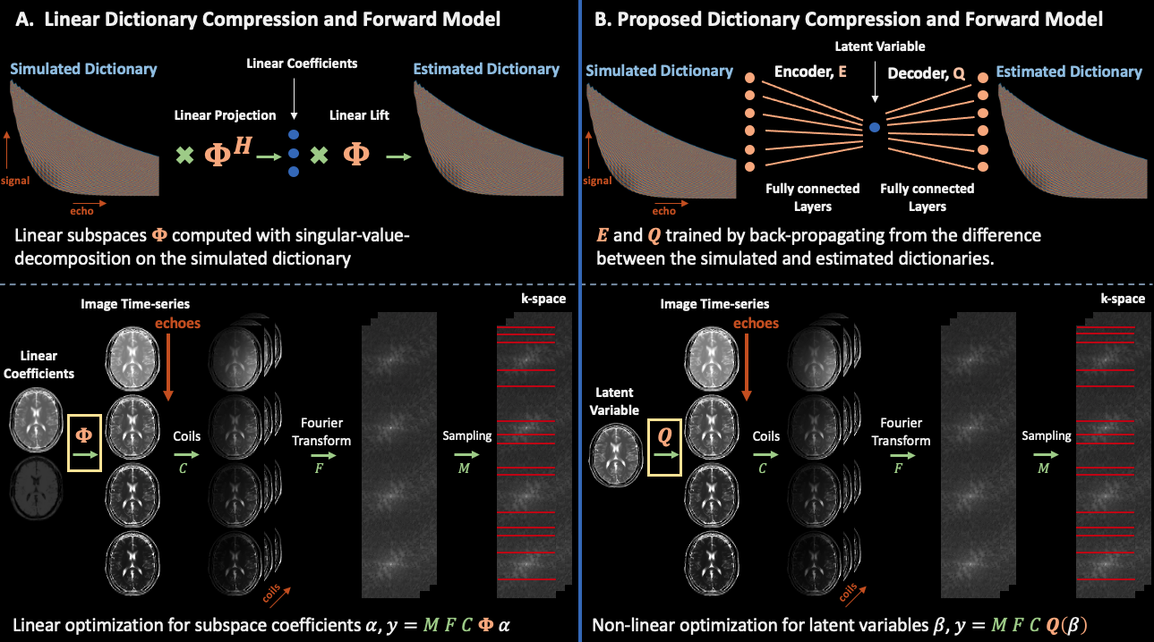
Figure 1: (a) The SVD generates a subspace from a dictionary of TSE signal evolution with 2-4 coefficients, while (b) the auto-encoder learns a representation of signal evolution with 1 latent variable. Inserting either the subspace or decoder in the forward model reduces the number of variables required to resolve signal dynamics. The auto-encoder’s more compact latent representation, compared to the subspace, enables improved reconstruction quality in subsequent experiments.
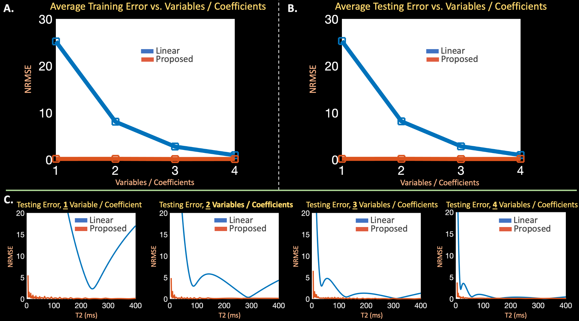
Figure 2: (a) + (b) Average error across the entire training and testing dictionaries of TSE signal evolution using linear subspaces and proposed auto-encoders with {1,2,3,4} coefficients or latent variables. (c) Error for individual signal evolutions, associated with different T2 values, in the testing dictionary using subspaces and auto-encoders. The subspace requires 3-4 coefficients, while the auto-encoder effectively captures signal evolution with just 1 latent variable.
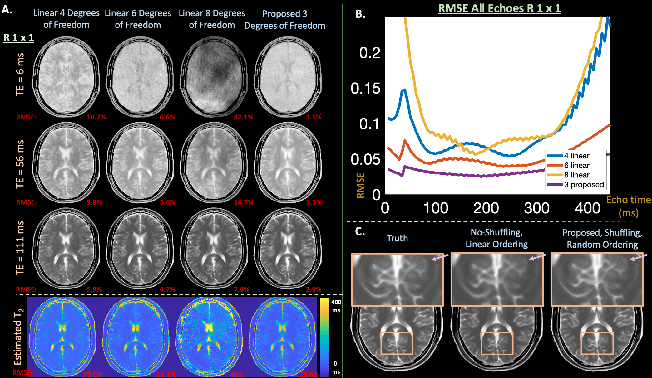
Figure 3: (a) Images, estimated T2 maps, and (b) RMSE plots vs.echo time from a simulated 3D T2-shuffling acquisition comparing the subspace and proposed reconstruction with {4,6,8} and 3 degrees of freedom respectively. The reduced degrees of freedom enabled by inserting the decoder into the T2-shuffling forward model yields cleaner images and lower RMSE. (c) Additionally, proposed maintains the improved sharpness characteristic of shuffling, in comparison to a non-shuffled reconstruction.
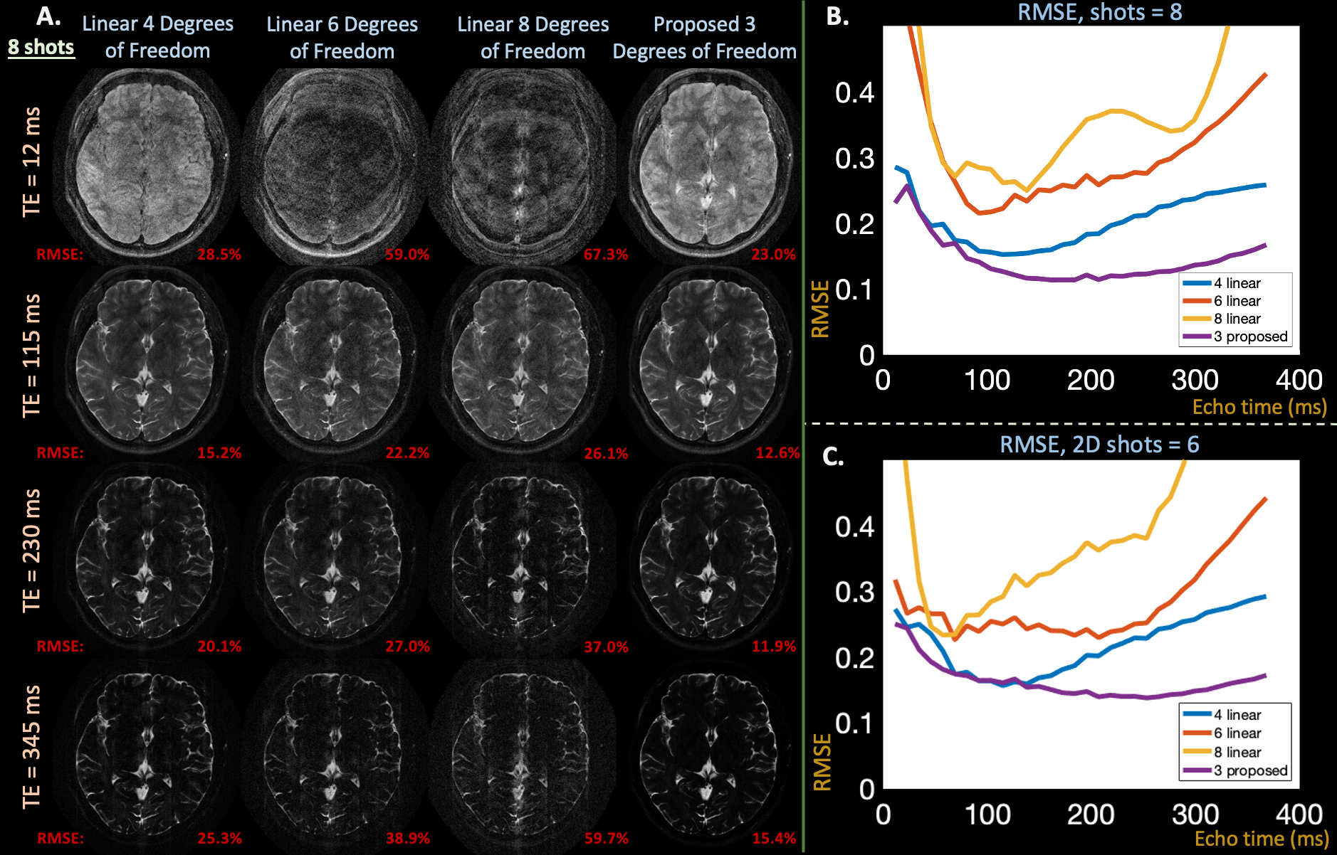
Figure 4: (a) Reconstructed images from an in-vivo, retrospective T2-shuffling acquisition at exemplar echo times comparing subspace constraints with {4,6,8} and the proposed approach with 3 degrees of freedom. (b) RMSE plots of reconstructed images at each echo time in signal evolution with retrospective 8 and (c) 6 shot acquisitions. Like in simulation, the proposed approach yields cleaner images, particularly at earlier echo times, and lower RMSE through reduced degrees of freedom.
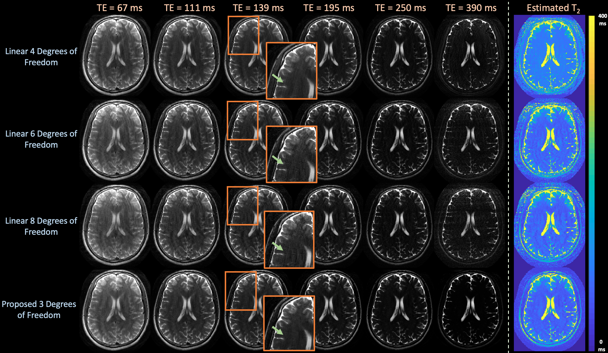
Figure 5: Images and estimated T2-maps from an in-vivo, prospective 2D T2-shuffling acquisition with 4 shots at exemplar echo times comparing linear subspace reconstructions with {4,6,8} and the proposed approach with 3 degrees of freedom. The proposed technique yields qualitatively cleaner images, as highlighted by the zoomed images and arrows, by employing a forward model with fewer degrees of freedom in comparison to the linear approach.
DOI: https://doi.org/10.58530/2022/0247