Introduction

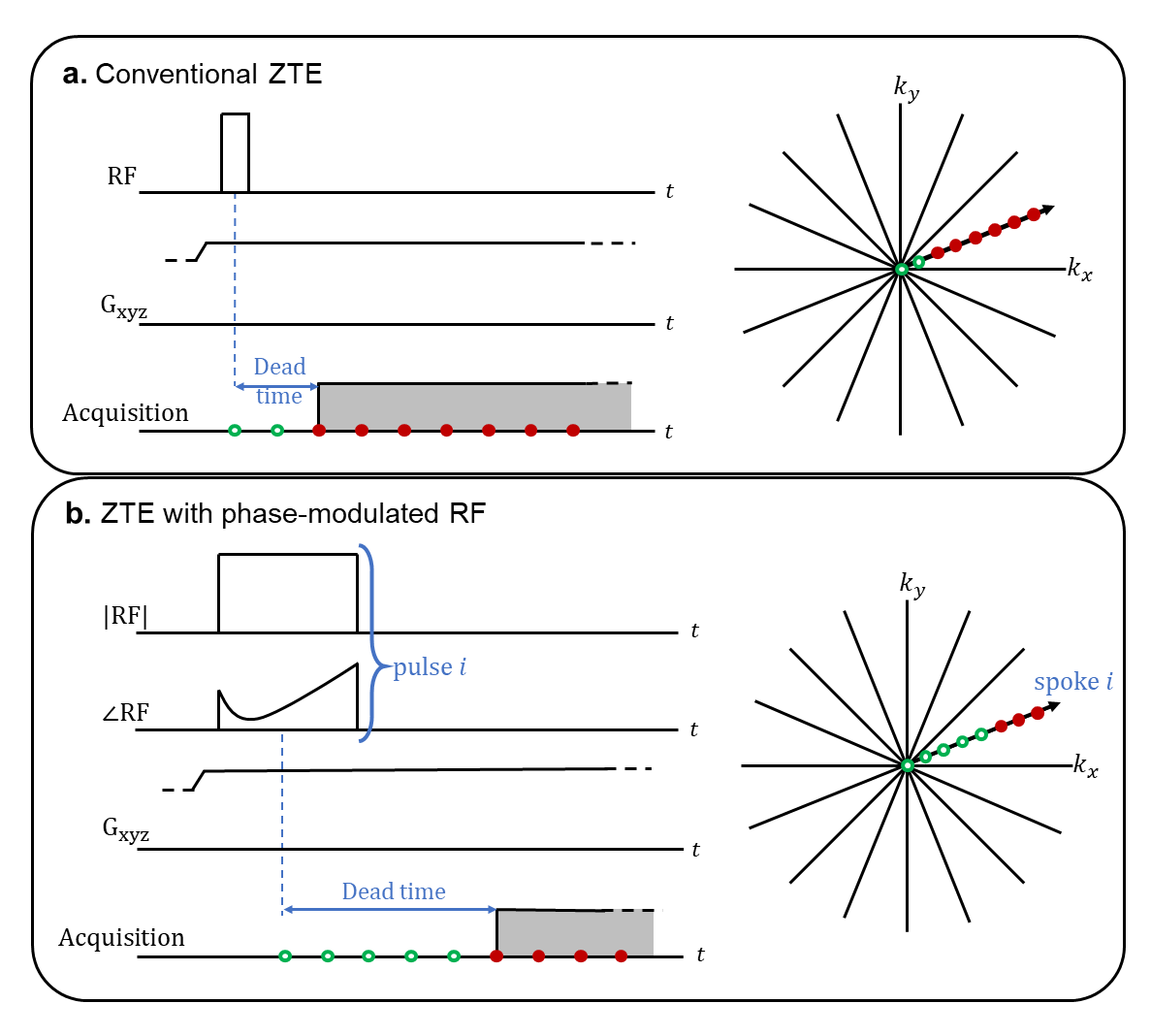
Zero echo time (ZTE) imaging, based on RUFIS¹, is a fast, silent, 3D technique. ZTE has a sampling efficiency suitable for rapid T1-weighted imaging since it does not require spoiling gradients, unlike comparable sequences such as FLASH². However, ZTE has native proton density contrast due to small flip angle excitation with short, hard RF pulses. Preparation segments are typically included to increase T1-weighting³, but these reduce time-efficiency due to necessary gradient ramp-down and inversion time waiting period. Alternatively, larger flip angle pulses increase T1-weighting. These pulses require high time-bandwidth products to excite the entire imaging volume in the presence of the readout gradient.

Previous approaches^4,5 achieve larger flip angles with longer frequency-swept pulses and recover dead-time gaps using algebraic reconstruction⁶. However, this formulation is constrained to sampling patterns with opposing spokes and radial oversampling. Additionally, algebraic reconstruction is limited to either small dead-time gaps⁶ or small T/R switch times⁵. Other dead-time infilling methods, like WASPI⁷ and PETRA⁸, require additional acquisitions with lower gradient strength. These methods require extra scan time and are not suitable for scans with motion or changing contrast. Therefore, we formulate an inverse problem to directly reconstruct an image from multi-coil k-space data without any intermediate dead time infilling.

Method

Our ability to recover large dead-time gaps is due to phase-modulated excitations and parallel imaging with 3D coil sensitivities. The excitation profiles and coil sensitivities apply image-domain weightings, which correspond to k-space convolutions that spread information between spatial frequencies. Hence, we can estimate missing dead-time samples using information mixed into higher acquired frequency locations.

Acquisition
We use quadratic phase-modulated (chirp) pulses, which are near-optimal for B1 power⁸, and achieve ~7$$$\pm$$$0.7$$$^{\circ}$$$flip angle. The chirp bandwidth is slightly greater than the imaging bandwidth to achieve flat excitation within 10% passband ripple. Similar to [5], we use two modulated chirps to improve inverse problem conditioning. However, we also use different sweep directions and alternate between the two pulses across odd/even TRs, instead of doubling scan time. Our method allows for any number of different excitations between TRs.

Formulation
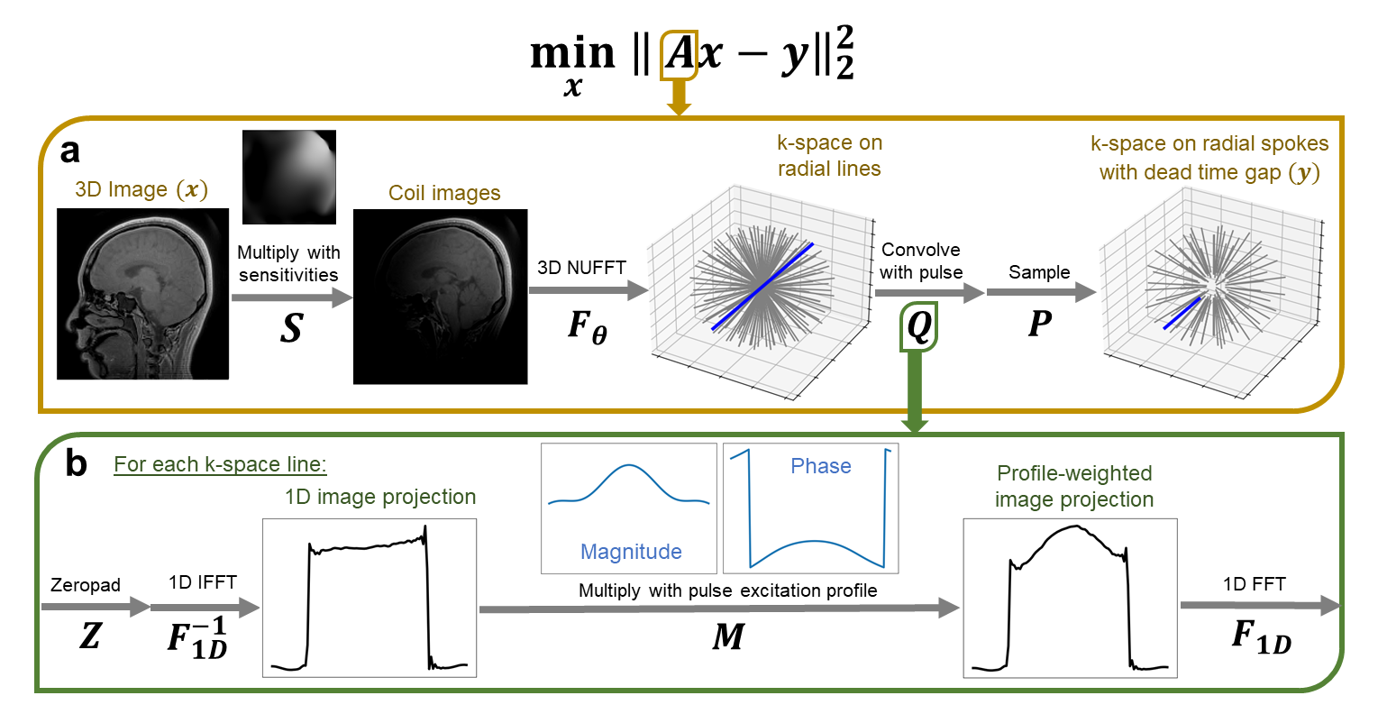
We formulate the inverse problem as a least squares minimization with an L1-wavelet regularization term as follows: $${\min}_x ||Ax-y||_2^2 + \lambda||\psi x||_1$$ Here, $$$x$$$ is the 3D image, $$$A$$$ is our forward model, $$$y$$$ is the multi-coil k-space data with dead-time gap, $$$\lambda$$$ is the regularization weight, and $$$\psi$$$ is the wavelet transform operator. We model the data acquisition forward operator as: $$A=P\cdot Q\cdot F_\theta \cdot S$$ As shown in Figure 2, $$$S$$$ is the multiplication with coil sensitivities, $$$F_\theta$$$ is the 3D NUFFT onto full-diameter radial lines, $$$Q$$$ is the 1D convolution of each line with the pulse waveform (implemented via DFT), and $$$P$$$ is the re-sampling onto radial spokes with the dead-time gap.
Since the gradient direction is constant for each TR, the 3D profile-weighting varies only in one direction¹¹ which allows us to apply the profile-weighting on a 1D image projection instead. This trick significantly reduces the computational overload of solving the inverse problem.

We iteratively solve this optimization problem using the Primal-Dual Hybrid Gradient algorithm¹², with step size parameters $$$\tau$$$ as the reciprocal of the maximum eigenvalue of $$$A$$$ (found using the power method), with $$$\sigma$$$ and $$$\theta$$$ as 1. After normalizing k-space data with respect to the 95^th percentile of the image, $$$\lambda$$$ was set to 0.1.

Simulations
We simulated multi-coil k-space data by running a 2D version of the forward model with realistic coil sensitivities. To avoid an “inverse crime”¹³, we used a phantom with an 8x higher resolution than the reconstruction. Complex random Gaussian noise was added to simulated k-space. Resulting image noise variance was estimated via 100 Monte-Carlo trials.

Experiments
We acquired phantom scans and a head scan of a healthy volunteer on a GE-3T MR750W (with $$$\pm$$$31.25kHz rBW, 2.4ms TR). We simulated alternated pulses by retrospectively interleaving odd/even TRs from two acquisitions with different excitations. This method eliminated possible steady-state disruptions from alternate pulses. We also discarded the first one or two samples along each acquired spoke due to significant ripple from the digital filter applied by the scanner receiver unit. Furthermore, we heuristically accounted for gradient delays by reconstructing on coordinates shifted by half-sample. Reconstructions were performed on a GeForceRTX GPU and took ~20min.

Results and Discussion

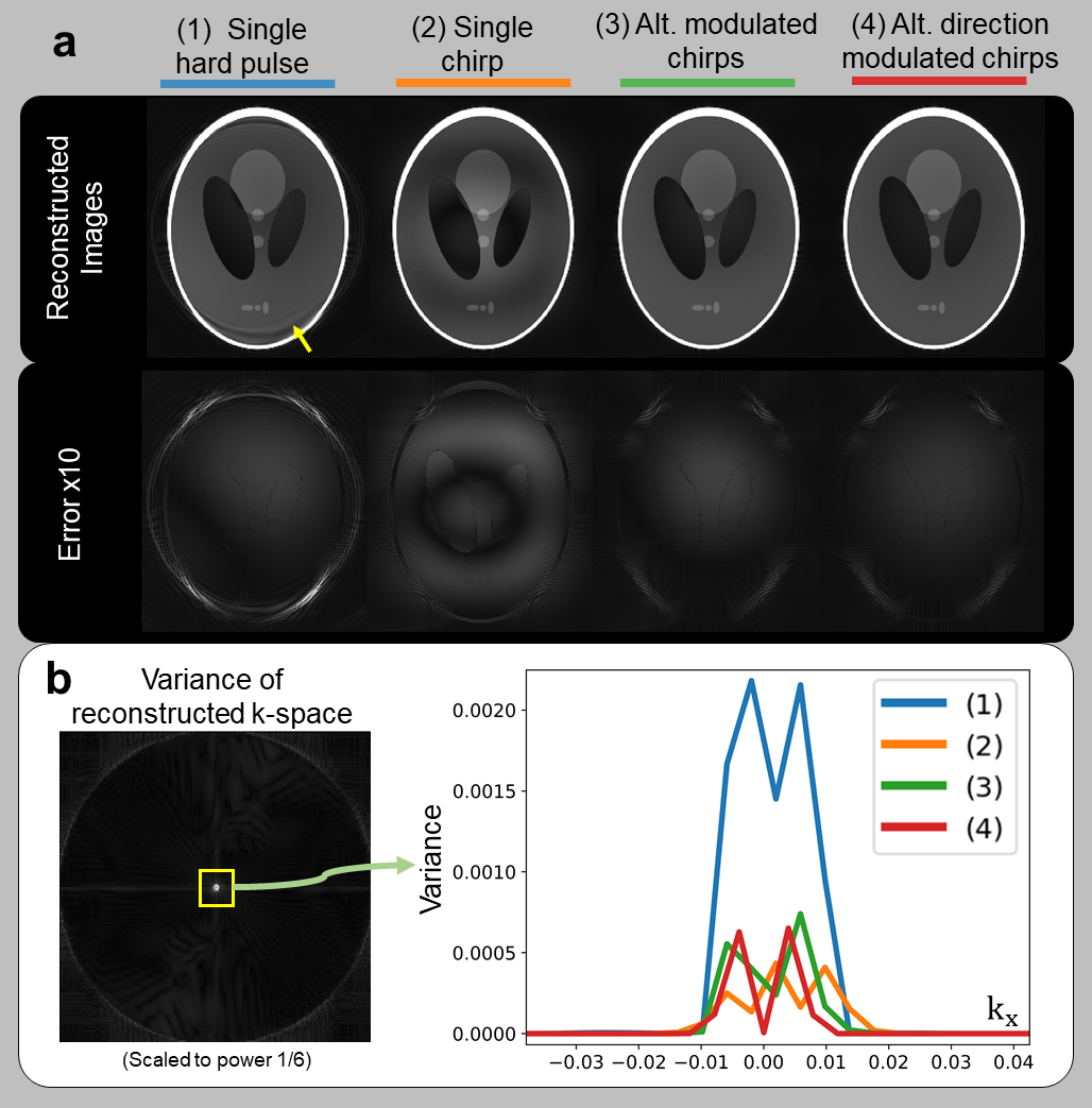
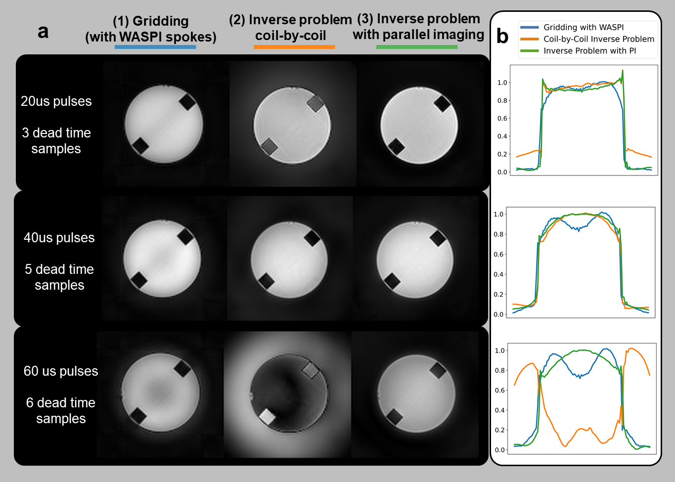
In Figure 3, we analyze conditioning for different pulses of the same duration(40us) using simulations. Reconstruction error appears as low-frequency image noise, depicted by higher variance near the k-space center. Alternating direction modulated chirps demonstrate the best conditioning within this experiment.

In Figure 4, we demonstrate how parallel imaging significantly improves conditioning by comparing to a coil-by-coil version of our inverse problem, as well as gridding with WASPI⁷ spokes. The inverse problem requires parallel imaging to recover large dead-time gaps, corroborating the findings in [14].

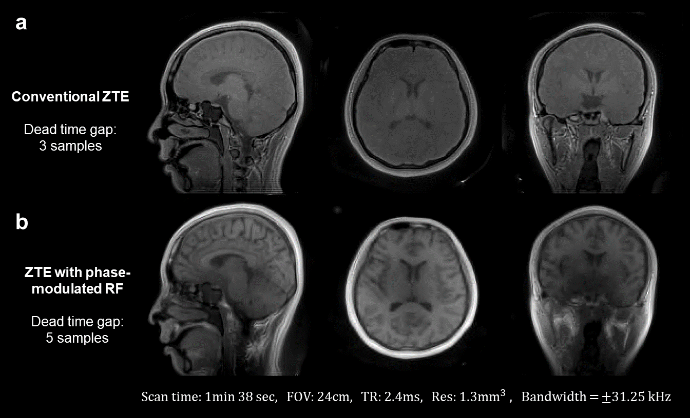
In Figure 5, we use alternated chirps and our inverse problem to reconstruct in-vivo images with significant T1 contrast. These images do contain some low-frequency variations and blurring, which is likely due to some model violations such as inaccurate pulse profiles and scanner digital filter ripple.

Conclusion

The proposed method introduces a parallel imaging, inverse problem-based formulation to reconstruct T1-weighted ZTE with phase-modulated excitations.

Acknowledgements

We would like to thank Florian Wiesinger for assistance with the ZTE pulse sequence and Gopal Nataraj for overall guidance. We would also like to thank Ekin Karasan for help with simulations.