Introduction

Imaging at higher field strengths benefits from increased SNR and is hence frequently used in fMRI^1-3. However, artefacts due to B₀ inhomogeneities are also more pronounced. If B₀ correction is performed, commonly a field map is acquired, requiring additional scan time, processing of the maps, and the maps are prone to dynamic effects like patient motion. Hence, estimation of B₀ maps is an intriguing challenge^4,5. Most of the proposed methods rely on dual acquisitions like EPI-up/down^4,6 and none is universally applicable. As an alternative, B₀ self-correction based on implicit temporal encoding by array detection has been shown feasible at 3T⁷.In this abstract, we explore the performance of this approach at 7T, show limitations of straight application as used for 3T and present improvements by constituting an adaptive basis.

Methods

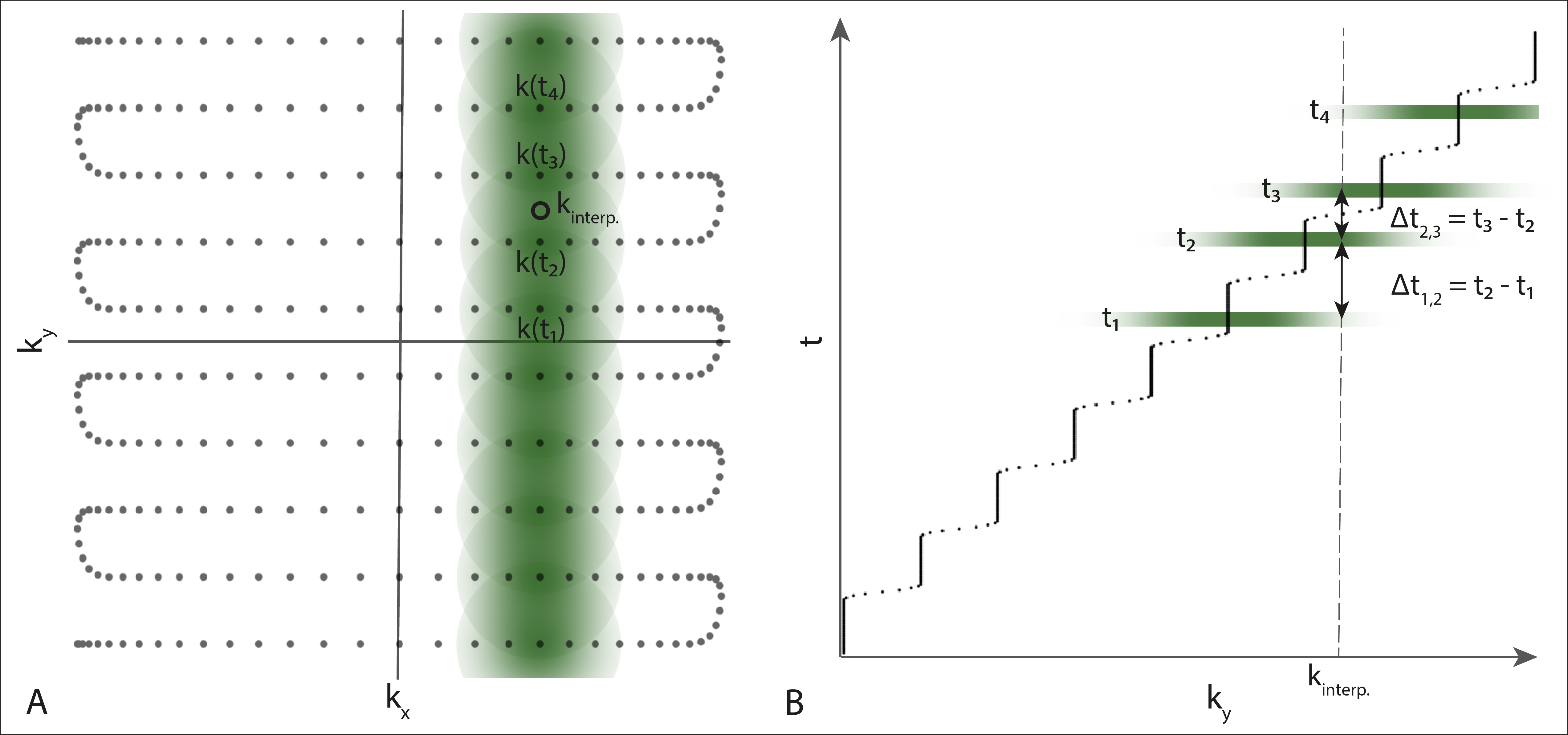
Joint Estimation of B₀ and the Object
Given a discretized signal equation$$\mathbf{m}=E(\mathbf{\Delta\omega_0})\mathbf{v}\;\;\;(1)$$with the measured signal$$$\;\mathbf{m}$$$, the encoding operator$$$\;E\;$$$incorporating field inhomogeneity$$$\;\mathbf{\Delta\omega_0}\;$$$and the object$$$\;\mathbf{v}$$$, joint reconstruction of$$$\;\mathbf{\Delta\omega_0}\;$$$and$$$\;\mathbf{v}\;$$$can be deployed as minimization:$$\mathcal{L}(\mathbf{\Delta\omega_0},\mathbf{v})=\Vert\,\mathbf{m}-E(\mathbf{\Delta\omega_0})\mathbf{v}\,\Vert^2.\;\;\;(2)$$B₀ information can be encoded implicitly by overlapping coil footprints of samples acquired at different times⁷, see Fig. 1.
Every minimum of the loss (2) is particularly optimal in$$$\;\mathbf{v}$$$, which is obtained by image reconstruction for given$$$\;\mathbf{\Delta\omega_0}$$$
$$\mathbf{v}=E^+(\mathbf{\Delta\omega_0})\mathbf{m}\;\;\;(3)$$Inserting (3) into (1) yields a loss solely depending on$$$\;\mathbf{\Delta\omega_0}$$$
$$\mathcal{L}(\mathbf{\Delta\omega_0)})=\Vert\,(Id-E(\mathbf{\Delta\omega_0})E^+(\mathbf{\Delta\omega_0}))\mathbf{m}\,\Vert^2\;\;\;(4)$$with the derivative with respect to$$$\;\mathbf{\Delta\omega_0}$$$
$$\nabla_{\Delta\omega_0}\mathcal{L}(\mathbf{\Delta\omega_0})=2\Re\{-i\text{diag}((E^+\mathbf{m})^H)E^H\text{diag}(t)(\mathbf{m}-EE^+\mathbf{m})\}.\;\;\;(5)$$To minimize (4), the algorithm is initialized with a zero field map and a gradient descent method is performed until convergence amounting to a non-convex step length determination⁷. As the algorithm yields B₀-corrected images without using any knowledge on B₀ it is called “B₀ self-correction”.

Regularization
The field map is modelled in a smooth basis with 2^nd order B-splines$$$\;\mathbf{\beta}\;$$$centered at positions$$$\;\mathbf{r}_j\;$$$
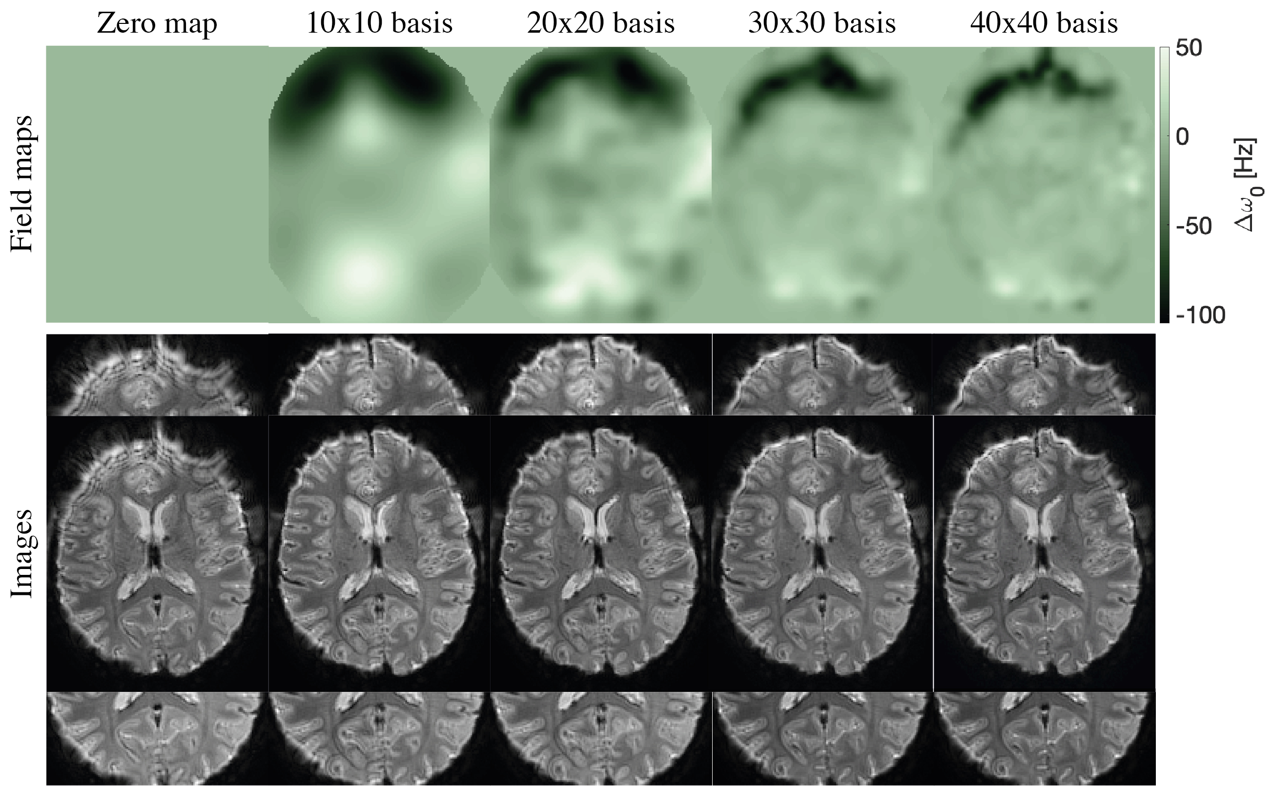
$$\mathbf{\Delta\omega_0}\approx\sum_jb_j\mathbf{\beta}_j.\;\;\;(6)$$reducing the number of parameters of the optimization. B₀ self-correction is performed modelling B₀ on equidistant grids of$$$\;10\times10$$$,$$$\;20\times20$$$,$$$\;30\times30$$$,$$$\;40\times40\;$$$grid points. Smaller numbers of basis functions lead to fewer parameters and result in stronger regularization, whereas higher numbers of basis functions allow depiction of finer details.
The linearity of the basis is beneficial as the gradient of the loss with respect to a basis coefficient is given by the dot product$$(\nabla_b\mathcal{L}(\mathbf{b}))_j=\mathbf{\beta}_j\cdot\nabla_{\Delta\omega_0}\mathcal{L}(\mathbf{\Delta\omega_0}).\;\;\;(7)$$

Basins of Attraction
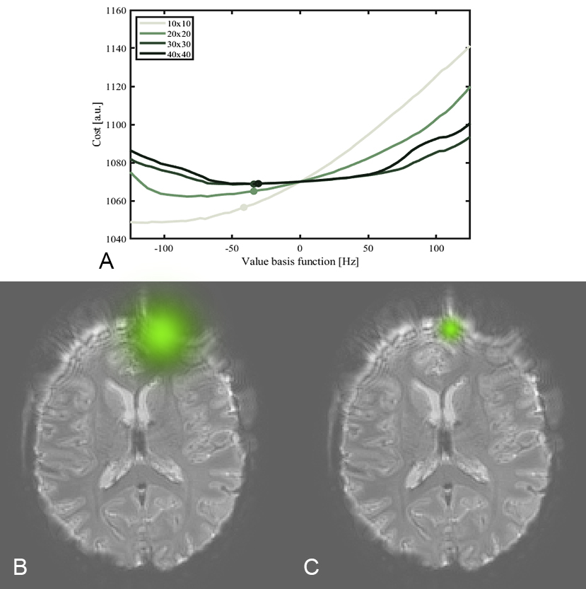
For non-convex optimization problems, the size of the basin of attraction of desired solutions is crucial to allow for uncertainty in the initialization. To investigate the influence of the number of basis functions on the loss, it is depicted for variation of one basis coefficient.

Adaptive Basis
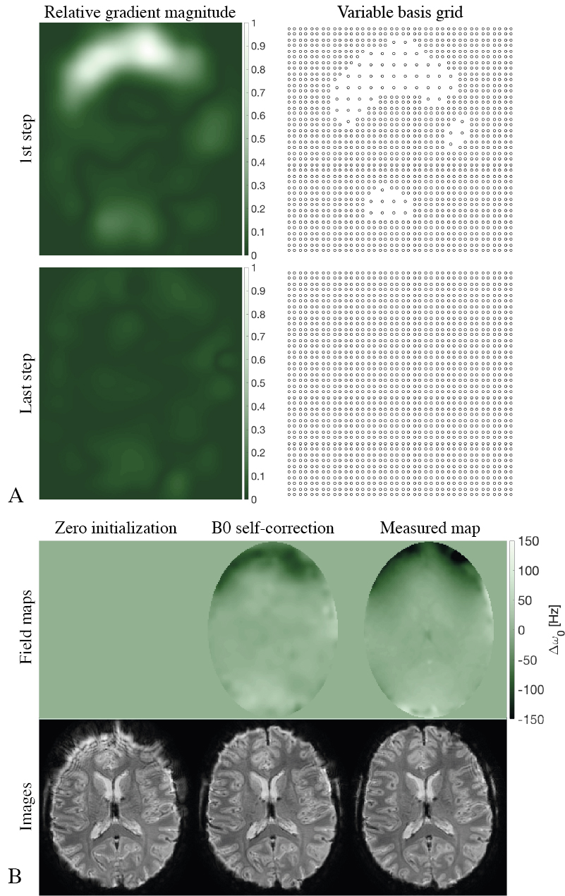
In regions of high B₀ offsets, distortions will be stronger requiring a higher degree of regularization. The field map, however, is a-priori not known but the gradient$$$\;\nabla_{\Delta\omega_0}\mathcal{L}(\mathbf{\Delta\omega_0})\;$$$is, which, in each optimization step, is only multiplied with a scalar. Consequently, relative variation in each descent step is given. Assuming the B₀ offset to be high in areas where the gradient is high, a variable density basis can be setup based on relative absolute gradient strengths. Variable bases used here are constituted of two equidistant bases with$$$\;20\times20\;$$$and$$$\;40\times40\;$$$grid points.

Measurements
Data was acquired on a 7T MR system (Philips Healthcare, Best, The Netherlands) using a$$$\;32$$$-channel head coil (Nova Medical, Wilmington, MA) equipped with$$$\;16\;$$$fluorine NMR field probes⁸ integrated in the set-up. Spiral-out imaging with$$$\;1.8\times1.8$$$,$$$\;1.3\times1.3$$$,$$$\;1.1\times1.1$$$,$$$\;1.0\times1.0\text{mm}^2\;$$$resolution for$$$\;\text{R}=1-4$$$,$$$\;\text{TE}=15\text{ms}$$$,$$$\;\text{FOV}=22\times22\text{cm}^2\;$$$was performed. Additionally, a two-echo GRE sequence was acquired to fit B₀ and B₁ maps.

Results

Number of Basis Functions
Performing B₀ self-correction with constant density bases leads to improved depiction quality and reasonable field map estimates, see Fig. 2. Remarkably, the correction worked better in the frontal part when choosing a coarser basis as there B₀ offsets are higher. However, the level of depiction is higher in the rear part for a finer basis. A trade-off for the basis resolution can be found between$$$\;20\times20\;$$$and$$$\;30\times30\;$$$coefficients.

Size of Basins of Attraction
For larger basis kernels, i.e. stronger regularization, the loss becomes smoother, but the minimum of the loss does not coincide with the optimal value, see Fig. 3A, presumably due to averaging B₀ over a wider range. For smaller basis kernels the optimal value coincides with the minimum of the loss but the size of the basin of attraction gets smaller and other local minima show up (Fig. 3A). These effects on the loss function motivate an adaptive basis strategy.

Adaptive Basis
B₀ self-correction is more challenging at higher field as the distortions are stronger. Employing a variable density basis results in B₀ self-corrected images (Fig. 4B) that are superior to images using constant bases. Leveraging information of the gradient to adjust the basis along the optimization leads to stronger regularization in highly off-resonant parts in the beginning, and a constant basis resolution in the last steps of the optimization (Fig. 4A).
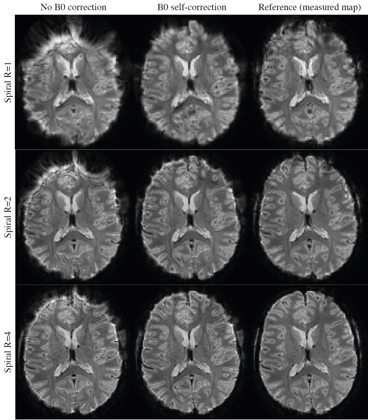
B₀ self-correction with a variable density basis shows consistent performance for spiral 7T images acquired with other acceleration factors (Fig. 5).

Discussion and Conclusion

Off-resonance self-correction at 7T was shown to be feasible. At 7T B₀ off-resonances are generally higher than at 3T, but the implicit encoding might benefit from the shorter wavelengths of the sensitivities. Variable density bases where shown to be effective to improve upon constant density bases. The algorithm is applicable to any trajectory but spirals were shown here as they form a particularly challenging task given the strong blurring artefacts.

Acknowledgements

The authors would like to thank Maria Engel for her support in acquiring the data.