0241
Deep Subspace Learning for Improved T1 Mapping using Single-shot Inversion-Recovery Radial FLASH
Moritz Blumenthal1, Xiaoqing Wang1,2, and Martin Uecker1,2,3
1Institute for Diagnostic and Interventional Radiology, University Medical Center Göttingen, Göttingen, Germany, 2DZHK (German Centre for Cardiovascular Research), Göttingen, Germany, 3Institute of Medical Engineering, Graz University of Technology, Graz, Austria
1Institute for Diagnostic and Interventional Radiology, University Medical Center Göttingen, Göttingen, Germany, 2DZHK (German Centre for Cardiovascular Research), Göttingen, Germany, 3Institute of Medical Engineering, Graz University of Technology, Graz, Austria
Synopsis
Subspace based reconstructions can be used for quantitative imaging. We extend the recently added neural network framework in BART to support non-Cartesian trajectories and linear subspace constraint reconstructions. The network is trained to reconstruct coefficient maps from single-shot radial FLASH inversion recovery acquisitions. T1 maps are estimated using pixel-wise fitting to the signal model. The reconstruction quality of the coefficient and T1 maps are improved compared to an $$$\ell_1$$$-Wavelet regularized reconstruction. The subspace constraint network can be used for any linear subspace constraint reconstruction.
Introduction
Deep neural networks have been proven to significantly improve reconstruction quality of undersampled k-space data. Physics-based neural networks1,2 reduce the amount of required training data by incorporating the linear forward model in the network architecture.For quantitative MRI, the underlying unknowns are the MR parameters (such as T1, T2). The signal evolutions depending on T1, T2 of different tissues can be approximated in a low-dimensional subspace. Thus, a linear reconstruction with subspace constraint can be performed to estimate pixel-wise signal evolution and quantitative maps via pixel-wise fitting.3
In this work, we combine linear subspace reconstruction with physics-based reconstruction networks. We extend the neural network framework4 in BART5 to support non-Cartesian sampling patterns as well as subspace-based reconstructions.
Theory and Methods
Subspace Reconstruction for Single-Shot T1 MappingThe signal evolution of an inversion recovery FLASH sequence is given by
$$\begin{aligned}S(t) = S_{SS} -(S_0-S_{SS})\exp{\frac{t}{T_1^*}}\,.&&(1)\end{aligned}$$
The signal evolutions for different physical parameter combinations of the relative steady state signal $$$S_{SS}/S_0$$$ and $$$T_1^*$$$ are highly correlated and can be approximated well in a low dimensional linear subspace. We have simulated signal curves as described in [6] and determined the four most significant basis coefficients (c.f. Fig. 1).
We define the subspace constrained linear forward model as
$$\begin{aligned}A=\mathcal{PFCB}: \mathbb{C}^{N_x\times N_y\times 4}\to\mathbb{C}^{N_{\mathrm{readout}}\times N_{\mathrm{inversion}} \times N_{\mathrm{coil}} \times N_{time}}\,,&&(2)\end{aligned}$$
i.e. the 4 coefficient maps are mapped to the $$$N_{\mathrm{coil}}$$$-k-space acquired during $$$N_{\mathrm{inversion}}$$$ inversions. In the forward model, $$$\mathcal{B}$$$ is the multiplication of the coefficient maps with the subspace basis, $$$\mathcal{C}$$$ is the multiplication with the coil sensitivity maps (CSM)s, $$$\mathcal{F}$$$ is the Fourier transform and $$$\mathcal{P}$$$ is the projection to the sampling pattern - in our case to a radial trajectory with $$$N_{\mathrm{time}}=1500$$$ spokes. We assign each spoke to an inversion time.
The forward model $$$A$$$ is used to formulate a regularized inverse problem which can be solved for the coefficient maps $$$\boldsymbol{x}$$$ given the k-space data $$$\boldsymbol{y}$$$, i.e.
$$\begin{aligned}\boldsymbol{x}=\underset{\boldsymbol{x}}{\operatorname{argmin}}\lVert\mathcal{PFCB}\boldsymbol{x}-\boldsymbol{y}\rVert_2^2 + \mathcal{R}(\boldsymbol{x})\,.&&(3)\end{aligned}$$ Here, $$$\mathcal{R}$$$ is a regularization term - for example joint $$$\ell_1$$$-Wavelet regularization. Given the coefficient maps $$$\boldsymbol{x}$$$, the signal evolution is obtained by $$$\mathcal{B}\boldsymbol{x}$$$, which in turn is fitted pixel-wise to the signal model to obtain the T1 map. For more details, we refer to the review in [6].
Neural Network Based Subspace Reconstruction
In this work, we replace the reconstruction in Eq. 3 by a neural network inspired by MoDL2. In each of the $$$N=5$$$ iterations, we update the current iterate $$$\boldsymbol{x}^n$$$ by
$$\begin{aligned}\boldsymbol{x}^{n+1}=\underset{\boldsymbol{x}}{\operatorname{argmin}}\lVert\mathcal{PFCB}\boldsymbol{x}-\boldsymbol{y}\rVert_2^2 + \lVert\boldsymbol{x}-\mathtt{Net}(\boldsymbol{x}^n)\rVert_2^2\,.&&(4)\end{aligned}$$ Here, $$$\mathtt{Net}$$$ is a ResNet enhancing the current reconstruction. We use a 64-channel complex-valued ResNet with five layers with four input and output channels (c.f. Fig 2c). Eq. 4 and its derivatives are computed using the conjugate gradient algorithm as proposed in [2].
We build our implementation on the newly added neural network framework in BART4,5. As the conjugate gradient solver is the computationally most expensive part, an efficient implementation is crucial. The normal equation operator $$$\mathcal{B}^H\mathcal{C}^H\mathcal{F}^H\mathcal{PFCB}$$$ is implemented using the nuFFT in BART which commutes $$$\mathcal{B}$$$ with $$$\mathcal{C}$$$ and $$$\mathcal{F}$$$. Then, the basis $$$\mathcal{B}$$$ is included in the point spread function (PSF), such that $$$\mathcal{B}^H\mathcal{C}^H\mathcal{F}^H\mathcal{PFCB}$$$ is computed using the Toeplitz trick.7,8 We precompute $$$\mathcal{B}^H\mathcal{PB}$$$ as well as the adjoint reconstruction $$$\boldsymbol{x}_{\mathrm{adj}}=(\mathcal{PFCB})^H\boldsymbol{y}$$$ for multiple use across different data-consistency (DC) blocks (c.f. Fig. 2a.) and training epochs.
Network Training
Training data is acquired from 9 volunteers at a Skyra 3T scanner (Siemens Healthcare GmbH, Erlangen, Germany) using an inversion-prepared radial FLASH acquisition with 30 inversions. For data augmentation, we extract 24 consecutive inversions using a sliding window approach. Each of these augmented k-space datasets was rotated differently. While the 24 inversion dataset was used to reconstruct a reference, six single-shot inversions were extracted as training input, resulting in 378 pairs of single-shot and 24-shot k-space data.
Data from all coils was compressed to $$$N_{\mathrm{coil}}=8$$$ virtual coils. Gradient delays were estimated using RING9 and CSMs were estimated using a subspace version of NLINV10.
Reference coefficient maps from the 24 inversion dataset were estimated by solving Eq. 3 without any regularization. For training, we use the product of CSMs and coefficient maps as target (c.f. Fig 2a) as it is independent of the estimated CSMs. We trained the network with $$$N=5$$$ unrolled iterations for 50 epochs.
Results
Fig. 3 shows a single-shot example reconstruction for a volunteer excluded during training. The reconstruction of the 3rd and 4th coefficient maps are improved compared to a joint $$$\ell_1$$$-Wavelet regularized reconstruction. The corresponding difference maps with respective to the reference are presented in Fig. 4. Quantitatively, the normalized MSE is reduced compared to the $$$\ell_1$$$-Wavelet reconstruction. Fig. 5 presents the T1 maps estimated from the respective reconstructions. The neural network based method recovers more detailed image structure compared to the $$$\ell_1$$$-Wavelet regularized one.Discussion and Conclusion
In this work, we trained a physics based neural network to perform linear subspace based reconstruction. The network we trained can exploit correlations between the coefficient maps and improves the image quality, especially of the 3rd and 4th coefficient maps.The improved estimated T1 map motivates to further investigate the effect on the multi-component analysis of the single-shot data.
Finally, we note that the subspace constrained neural network can also be used to improve other subspace based reconstructions.
Acknowledgements
We acknowledge funding by the "Niedersächsisches Vorab" funding line of the Volkswagen Foundation.This work was supported by the DZHK (German Centre for Cardiovascular Research) and funded in part by NIH under grant U24EB029240.
References
1. K. Hammernik et al., “Learning a variational network for reconstruction of accelerated MRI data”, Magn. Reson. Med., vol. 79, no. 6, pp. 3055–3071, 20182. H. K. Aggarwal, M. P. Mani, and M. Jacob, “MoDL: Model-Based Deep Learning Architecture for Inverse Problems”, IEEE Transactions on Medical Imaging, vol. 38, no. 2, pp. 394–405, 2019
3. J. Pfister, M. Blaimer, W. H. Kullmann, A. J. Bartsch, P. M. Jakob and F. A. Breuer, "Simultaneous T1 and T2 measurements using inversion recovery TrueFISP with principle component-based reconstruction, off-resonance correction, and multicomponent analysis", Magn. Reson. Med. vol. 81, pp. 3488–3502, 2019
4. M. Blumenthal and M. Uecker, "Deep, Deep Learning with BART", ISMRM Annual Meeting 2021, In Proc. Intl. Soc. Mag. Reson. Med. 29;1754, 2021
5. M. Uecker et al., "BART Toolbox for Computational Magnetic Resonance Imaging", Zenodo, DOI: 10.5281/zenodo.592960
6. X. Wang, Z. Tan, N. Scholand, V. Roeloffs, and M. Uecker, “Physics-based Reconstruction Methods for Magnetic Resonance Imaging,” Philos. Trans. R. Soc. A., vol. 379, no. 2200, 2021.
7. M. Mani, M. Jacob, V. Magnotta, and J. Zhong, “Fast iterative algorithm for the reconstruction of multishot non-cartesian diffusion data,” Magn. Reson. Med., vol. 74, no. 4, Art. no. 4, 2015
8. J. I. Tamir, M. Uecker, W. Chen, P. Lai, M. T. Alley, S. S. Vasanawala and M. Lustig, “T2 shuffling: Sharp, multicontrast, volumetric fast spin-echo imaging,” Magn. Reson. Med., vol. 77, no. 1, 2017
9. S. Rosenzweig, H. C. M. Holme, and M. Uecker, “Simple auto-calibrated gradient delay estimation from few spokes using Radial Intersections (RING),” Magn. Reson. Med., vol. 81, no. 3, 2019
10. M. Uecker, T. Hohage, K. T. Block, and J. Frahm, “Image reconstruction by regularized nonlinear inversion-joint estimation of coil sensitivities and image content,” Magn. Reson. Med., vol. 60, no. 3, pp. 674-682, 2008
Figures
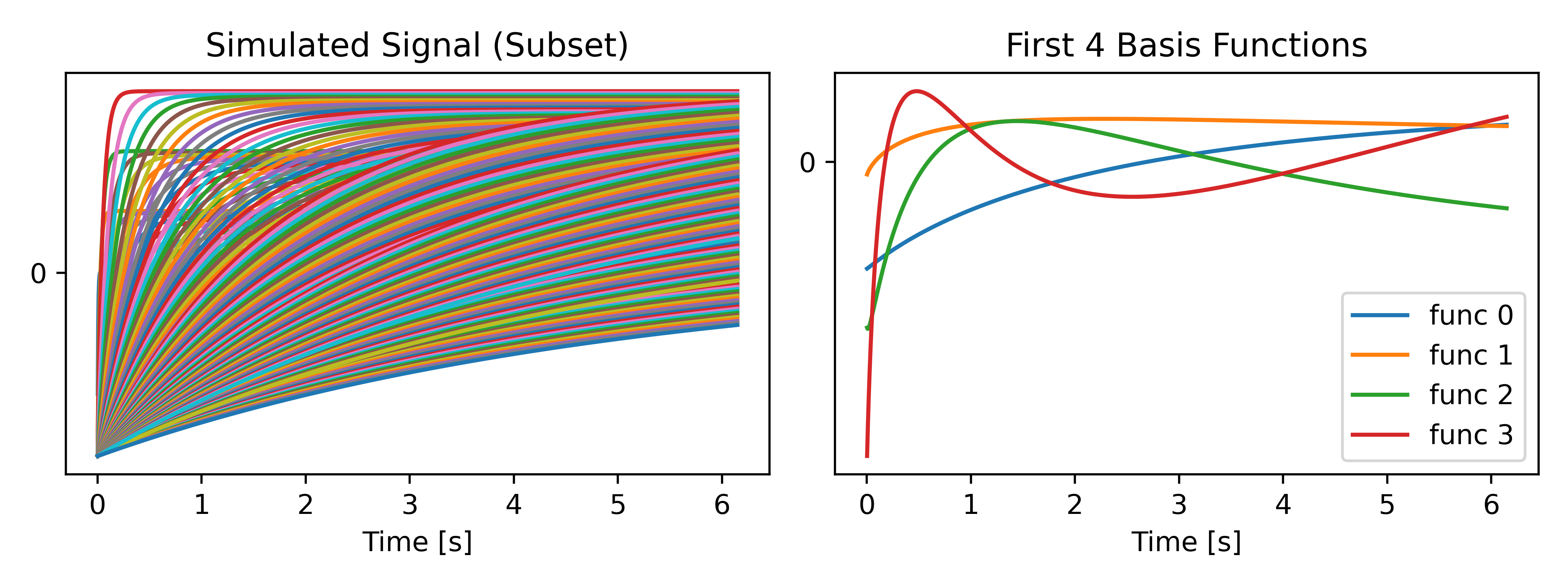
Fig 1: (Left) Simulated T1 relaxation curves (subset) and (Right) plot of the first 4 principal components following the PCA transform of the T1 dictionary.
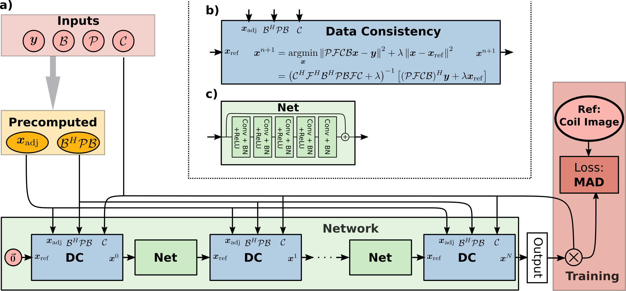
Fig. 2: a) Network structure of RecoNet for linear subspace constrained reconstruction. The adjoint (gridded) reconstruction $$$\boldsymbol{x}_{\mathrm{adj}}$$$ and $$$\mathcal{B}^H\mathcal{PB}$$$ on the Cartesian grid are precomputed for multiple use in the DC blocks. The output coefficient maps are multiplied with the CSM to compute the coil images used in the loss function. b) DC-block with non-Cartesian trajectory and temporal basis support. c) 64-channel complex-valued ResNet with one input/output channel per coefficient map.
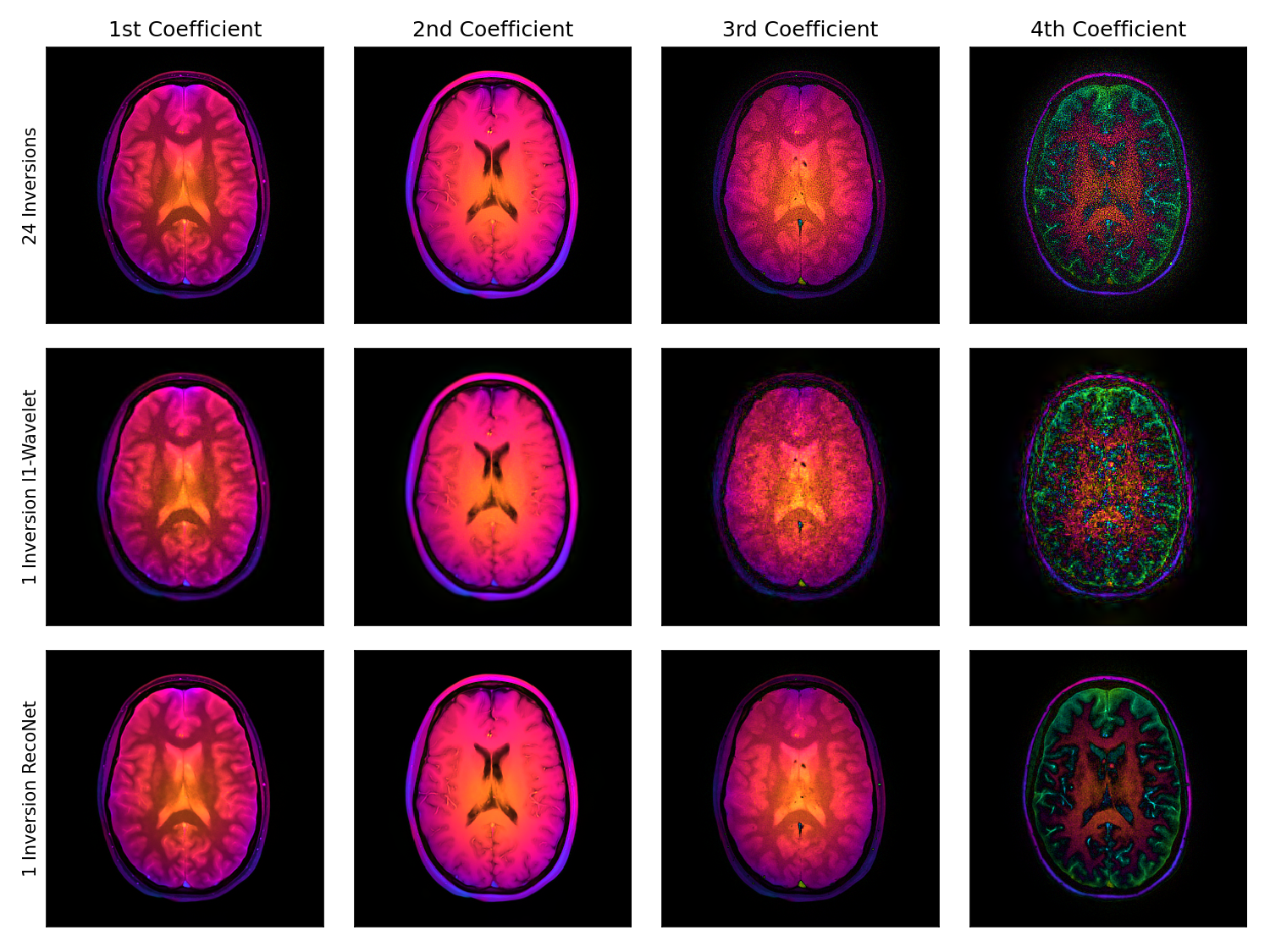
Fig. 3: Subspace coefficient maps of the first virtual coil reconstructed from (top) a dataset with 24 inversions, (middle) single-shot dataset using $$$\ell_1$$$-Wavelet regularization and (bottom) single-shot dataset using RecoNet. The phase is encoded by the color. The magnitude is normalized column-wise, i.e. the energy in the 4th coefficient map is significantly smaller than the first. RecoNet is capable of reconstructing the 3rd and 4th coefficient maps with less noise in comparison to the $$$\ell_1$$$-Wavelet regularized reconstruction.

Fig. 4: Difference between the 24-inversion coefficient maps and the respective single shot reconstructions in Fig. 3. The normalized mean squared error is computed over all coil images. RecoNet has a smaller reconstruction error compared to the $$$\ell_1$$$-Wavelet reconstruction.
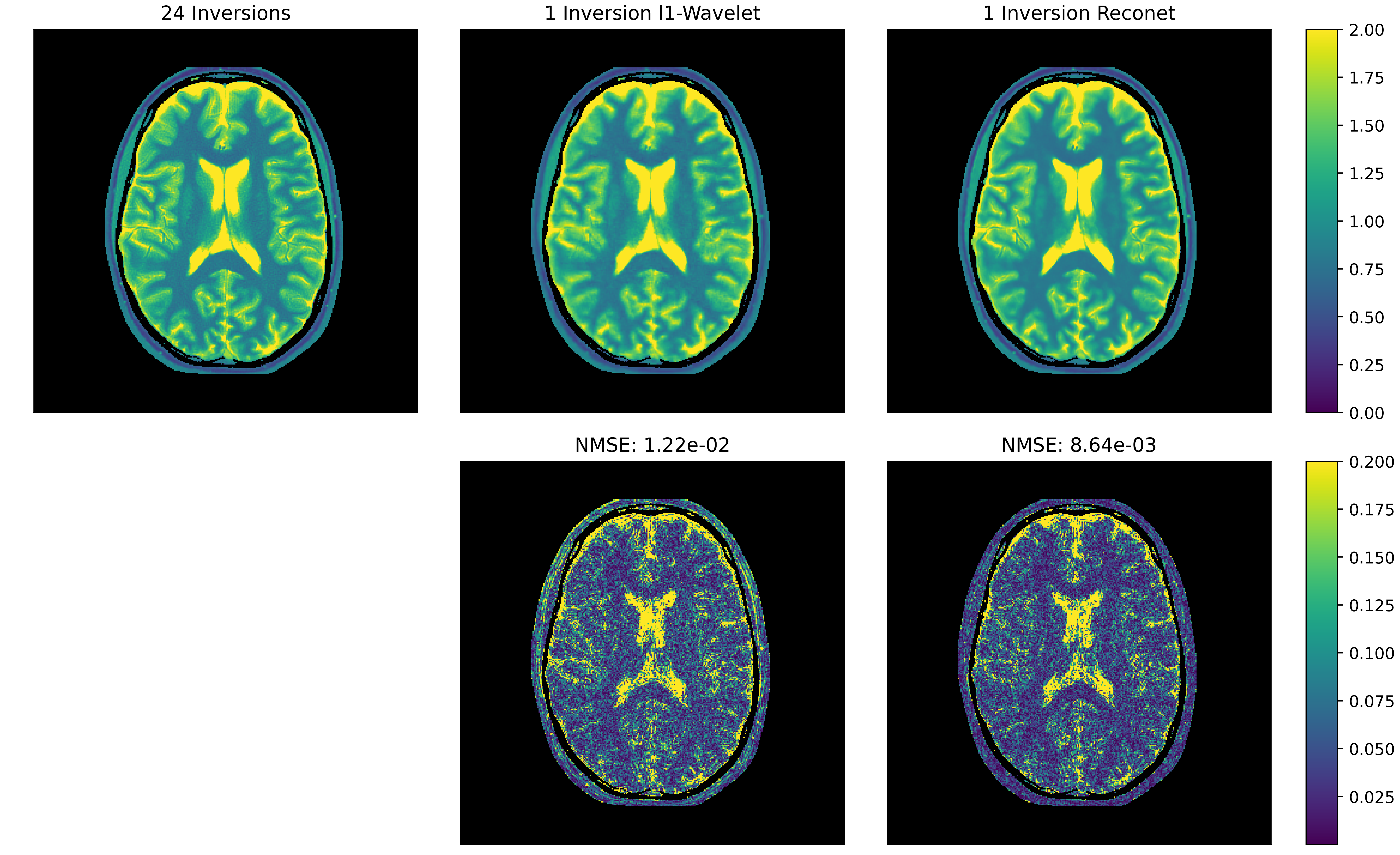
Fig. 5: T1 maps obtained from the 24 inversions dataset and the single-shot datasets using the respective subspace reconstructions as shown in Fig. 3.
DOI: https://doi.org/10.58530/2022/0241