0235
FieldMapNet MRI: Learning-based mapping from single echo time BOLD fMRI data to fieldmaps with model-based image reconstruction1Electrical Engineering and Computer Science, University of Michigan, Ann Arbor, MI, United States, 2Biomedical Engineering, University of Michigan, Ann Arbor, MI, United States
Synopsis
Artifacts due to B0 field off-resonance result in image distortions and blurring in non-Cartesian acquisitions. FieldMapNet is a learning-based method to map from each image in a spiral-in BOLD fMRI acquisition to a corresponding B0 fieldmap at that timepoint. We train FieldMapNet in a supervised fashion using custom data acquired at three echo times to generate ground truth dynamic fieldmaps. We then perform a tailored B0 correction at each fMRI timepoint using a model-based image reconstruction (MBIR). We show improved image space RMSE using FieldMapNet vs. a separately acquired GRE fieldmap, and a reduction in distortion artifacts and blurring.
Introduction
Off-resonance artifacts in MRI lead to geometric distortions and blurring for non-Cartesian acquisitions. Model-based image reconstruction (MBIR) using accurate fieldmaps can correct for these effects1, but such fieldmaps conventionally require a multi-echo acquisition and are often done separately before acquiring fMRI data. However, for dynamic imaging such as BOLD fMRI, having a fieldmap for every timepoint could improve image quality, especially in changing $$$B_0$$$ fields due to respiration or motion. Prior work has shown off-resonance correction on individual images using an entropy metric2, a piecewise linear estimate3, or with convolutional neural networks (CNNs)4,5. Here we use a residual UNet, called FieldMapNet, that, given a prior estimate of the fieldmap and image phase from an earlier timepoint, dynamically estimates fieldmaps from the phase of each timeseries image. The fMRI timeseries is then corrected using MBIR6, reducing the effects of potential network artifacts on the final images.Methods
MRI AcquisitionWe acquired human in vivo data for network training and test fMRI experiments on a 3T GE MR750 scanner with a Nova 32-channel head coil using the TOPPE pulse sequence programming language7. For both sets of data we acquired 80 slices of 2D single-shot fully sampled spiral-in images, with volume FOV=240×240×240mm3 and resolution=3×3×3mm3 (matrix size=80×80×80). We also acquired a conventional GRE field map (1:37s) prior to acquiring the spiral-in data.
Multiecho Training Data Parameters: To create the dynamic ground-truth off-resonance maps used for training the network, we acquired three sequential spiral-in images at each slice with TE=26.7/27.7/28.9ms ($$$\Delta$$$TE=1,2.3ms), FA=10°, volume TR=9.9s, # frames=20 (3:18min).
Testing Data Parameters: TE=26.7ms, volume TR=3.1s, # frames=65 (3:21min), FA=84°. The experiment was repeated with deep breathing to investigate the impact of large changes in off-resonance.
FieldMapNet Structure
FieldMapNet (Fig. 1) maps 5 input channels, $$$[\cos (\boldsymbol{\phi}_n^{TE1}), \sin (\boldsymbol{\phi}_n^{TE1}), \cos (\boldsymbol{\phi}_0^{TE1}), \sin (\boldsymbol{\phi}_0^{TE1}), \boldsymbol{\omega}_0]$$$ to a single output of $$$\boldsymbol{\omega}_n$$$, where $$$\boldsymbol{\phi}_n^{TE1}$$$ is the phase of the first TE image at timepoint $$$n$$$, $$$\boldsymbol{\phi}_0^{TE1}$$$ is the phase of the first TE image at some initial timepoint, $$$\boldsymbol{\omega}_0$$$ is a fieldmap calculated from $$$\boldsymbol{\phi}_0^{TE1}$$$, $$$\boldsymbol{\phi}_0^{TE2}$$$, and $$$\boldsymbol{\phi}_0^{TE3}$$$, and $$$\boldsymbol{\omega}_n$$$ is the fieldmap at timepoint $$$n$$$. We use cosine and sine of the phase to accommodate phase wraps. For the three-TE training data we used the first volume for $$$\phi_0^{TE1}$$$ and $$$\boldsymbol{\omega}_0$$$, and for the single-echo time test data we used the last timepoint from the most recent training data scan (this prior fieldmap takes 9.9s to acquire and could also be added to be beginning of the single-TE scan). We used a residual single-level UNet by passing $$$\boldsymbol{\omega}_0$$$ to the output as a skip connection, with 5×5 convolutional filters, MAE loss , learning rate=10-4, and the Adam optimizer, implemented in Keras.
FieldMapNet Training Data
We reconstructed images from the three TE data using a model-based image reconstruction (MBIR) as described in the section below. The images from the three TEs were used to calculate the fieldmaps $$$\boldsymbol{\omega}_n$$$ at each frame using a regularized iterative algorithm8. We used 10 subjects for network training and two subjects unseen by the network for testing. For training we selected slices within the brain region of the imaging volume, yielding 176 slices across all subjects, and 3520 unique image to fieldmaps pairs (from the 20 frames). We augmented the data using translations, rotations, and random bulk phase, leading to 22528/5632 training/validation pairs.
Model-based Image Reconstruction
Images at each timepoint are generated from an edge-preserving regularized reconstruction using a second-order finite difference operator, $$$\boldsymbol{C}$$$, and a Fair potential function $$$\psi$$$. The forward model, $$$\boldsymbol{A}$$$, includes sensitivity maps calculated using the sigpy.mri9 implementation of joint-sense10,11, a gridding operator, and the fieldmap $$$\boldsymbol{\omega}$$$6
$$ \boldsymbol{\hat{x}} = \mathop{\mathrm{arg\,min}}_{\boldsymbol{x}} \frac{1}{2} \| \boldsymbol{A}(\boldsymbol{\omega}) \boldsymbol{x}-\boldsymbol{y} \|_2^2+\beta R(\boldsymbol{x}) \hspace{10pt} \text{where} \hspace{10pt} R(\boldsymbol{x})=\sum_k \psi ([\boldsymbol{Cx}]_k)$$
with $$$\beta$$$ empirically set to 30. The images are first reconstructed using the GRE fieldmaps, and these images are input to FieldMapNet. Dynamic fieldmaps are then generated from the network and the images are re-reconstructed with the fieldmap at that timepoint. All reconstructions used the MATLAB implementation of MIRT12. Fig. 2 gives an overview of the method. This approach mitigates potential network hallucinations affecting the image by using a physics-based reconstruction as the final step.
Results
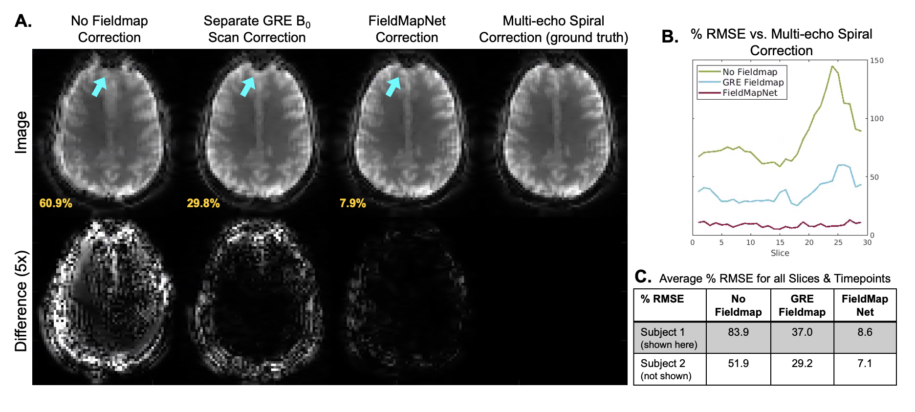
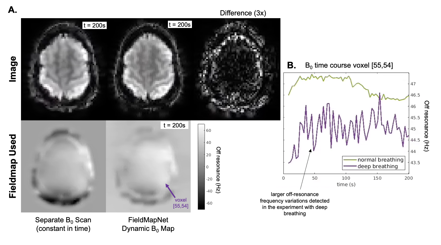
Fig. 3 shows fieldmaps generated using the iterative three-echo model-based method8 (ground truth) and the proposed FieldMapNet. Fig. 4A shows image reconstruction results compared to the 3-TE ground truth, Fig. 4B shows the % RMSE across slices, and Fig. 4C shows the summary statistics. Fig. 5A shows image results from the deep breathing experiment, reconstructed using the standard GRE fieldmap versus the dynamic fieldmaps from FieldMapNet, with reduced blurring using FieldMapNet. Fig. 5B shows the changes in B0 over the course of the scan detected by FieldMapNet, with more off-resonance detected in deep breathing vs. normal breathing, as expected.Discussion & Conclusions
We have demonstrated the potential to dynamically estimate a fieldmap from a single TE image using a prior fieldmap estimate and a residual one-level UNet. Using FieldMapNet with MBIR can correct for off-resonance while avoiding ML artifacts in the final image. We expect this method to improve the quality of fMRI experiments, especially in moving subjects where the fieldmap can change as a subject moves through the FOV.Acknowledgements
This work was supported by the National Institutes of Health Grants U01EB026977 and F32EB029289.References
1. K. Sekihara, M. Kuroda, and H. Kohno. Image restoration from non-uniform magnetic field influence for direct Fourier NMR imaging. Physics in Medicine and Biology, 29(1):15–24, 1984.
2. Douglas C. Noll, John M. Pauly, Craig H. Meyer, Dwight G. Nishimura, and Albert Macovskj.Deblurring for non-2D fourier transform magnetic resonance imaging. Magnetic Resonance inMedicine, 25(2):319–333, 1992.
3. Travis B. Smith and Krishna S. Nayak. Automatic off-resonance correction in spiral imagingwith piecewise linear autofocus. Magnetic Resonance in Medicine, 69(1):82–90, 1 2013.
4. David Y. Zeng, Jamil Shaikh, Signy Holmes, Ryan L. Brunsing, John M. Pauly, Dwight G.Nishimura, Shreyas S. Vasanawala, and Joseph Y. Cheng. Deep residual network for off-resonance artifact correction with application to pediatric body MRA with 3D cones. MagneticResonance in Medicine, 82(4):1398–1411, 10 2019.
5. Yongwan Lim, Yannick Bliesener, Shrikanth Narayanan, and Krishna S. Nayak. Deblurring forspiral real-time MRI using convolutional neural networks. Magnetic Resonance in Medicine,84(6):3438–3452, 2020.
6. Bradley P Sutton, Douglas C Noll, and Jeffrey A Fessler. Fast, Iterative Image Reconstruction for MRI in the Presence of Field Inhomogeneities. IEEE Transactions on Medical Imaging,22(2):178–188, 2003.
7. Jon Fredrik Nielsen and Douglas C. Noll. TOPPE: A framework for rapid prototyping of MR pulse sequences. Magnetic Resonance in Medicine, 79(6):3128–3134, 2018.
8. Amanda K. Funai, Jeffrey A. Fessler, Desmond T.B. Yeo, Douglas C. Noll, and Valur T. Olafsson. Regularized field map estimation in MRI. IEEE Transactions on Medical Imaging,27(10):1484–1494, 2008.
9. https://sigpy.readthedocs.io/en/latest/generated/sigpy.mri.app.JsenseRecon.html#sigpy.mri.app.JsenseRecon.
10. Leslie Ying and Jinhua Sheng. Joint image reconstruction and sensitivity estimation in SENSE(JSENSE). Magnetic Resonance in Medicine, 57(6):1196–1202, 2007.
11. Martin Uecker, Thorsten Hohage, Kai Tobias Block, and Jens Frahm. Image reconstruction by regularized nonlinear inversion - Joint estimation of coil sensitivities and image content. Magnetic Resonance in Medicine, 60(3):674–682, 2008.
12. https://github.com/JeffFessler/mirt
Figures
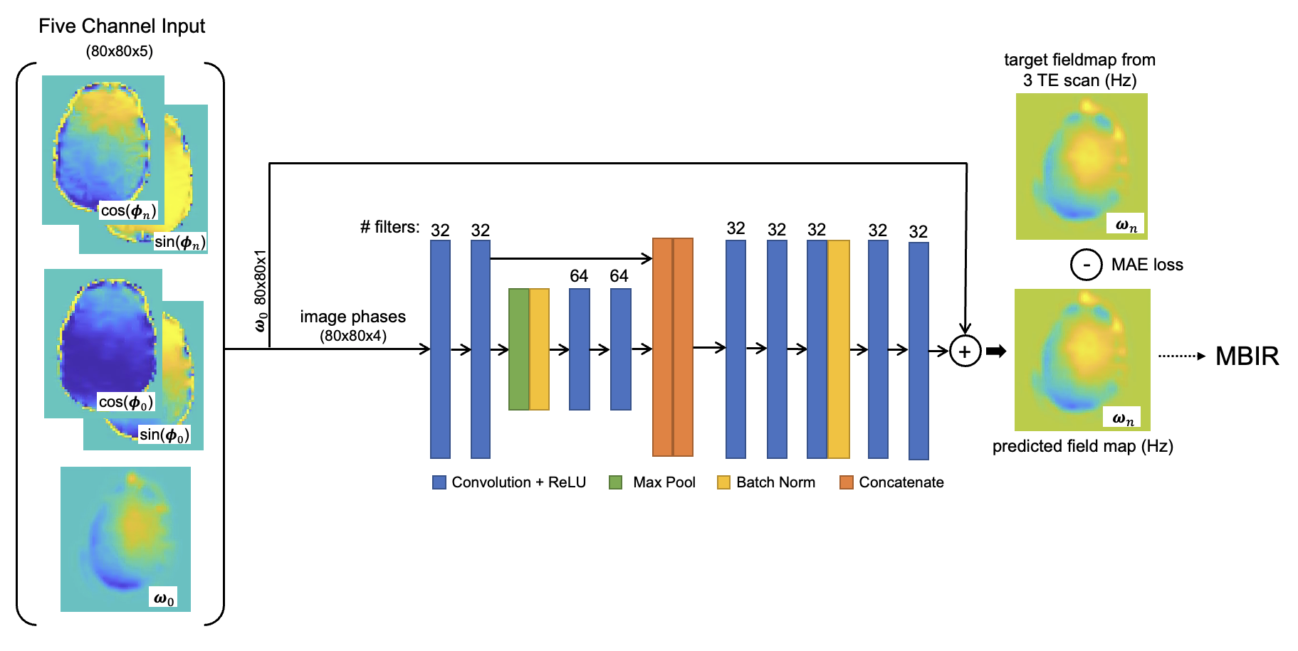
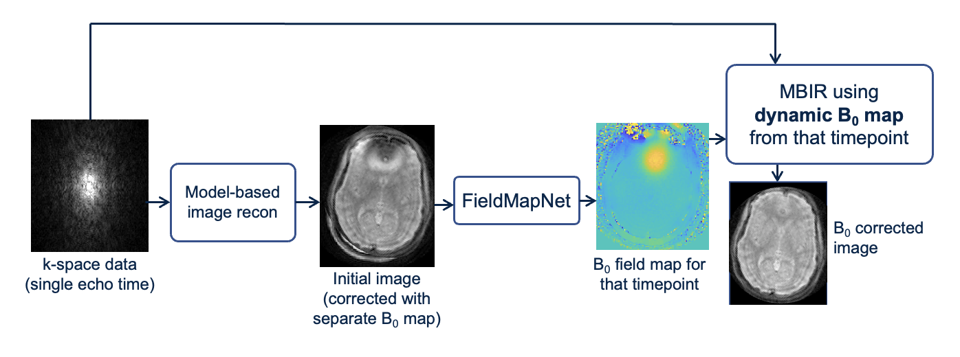
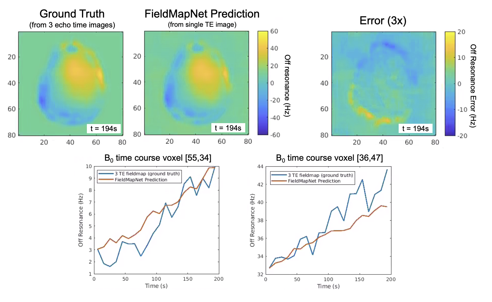
Figure 3. FieldMapNet Dynamic Off-resonance Estimates Compared to Ground Truth. Top Left: Ground truth fieldmap calculated using all three echo time images. Top Middle: FieldMapNet estimate calculated using a single echo time image. Top Right: Difference image, scaled by 3x. Bottom row shows the off-resonance for two voxels over the course of the scan.