Introduction

We recently proposed a self-learning framework to discover MRI sequences based on an MRI physics simulation, which was dubbed MRzero as zero sequence programming experience was provided, but only the Bloch equations¹. Here, we want to investigate if self-learning is also possible without having any model or simulation at hand, by exploring a subset of the MR sequence parameter space directly at a real MRI scanner. Thus we call this agent MR-double-zero. To mimic a real discovery of a novel MRI effect, we assume that we know about water relaxation and have relaxation-weighted sequences, but that CEST effects are still unknown and will be discovered by the MR-double-zero agent.

Methods

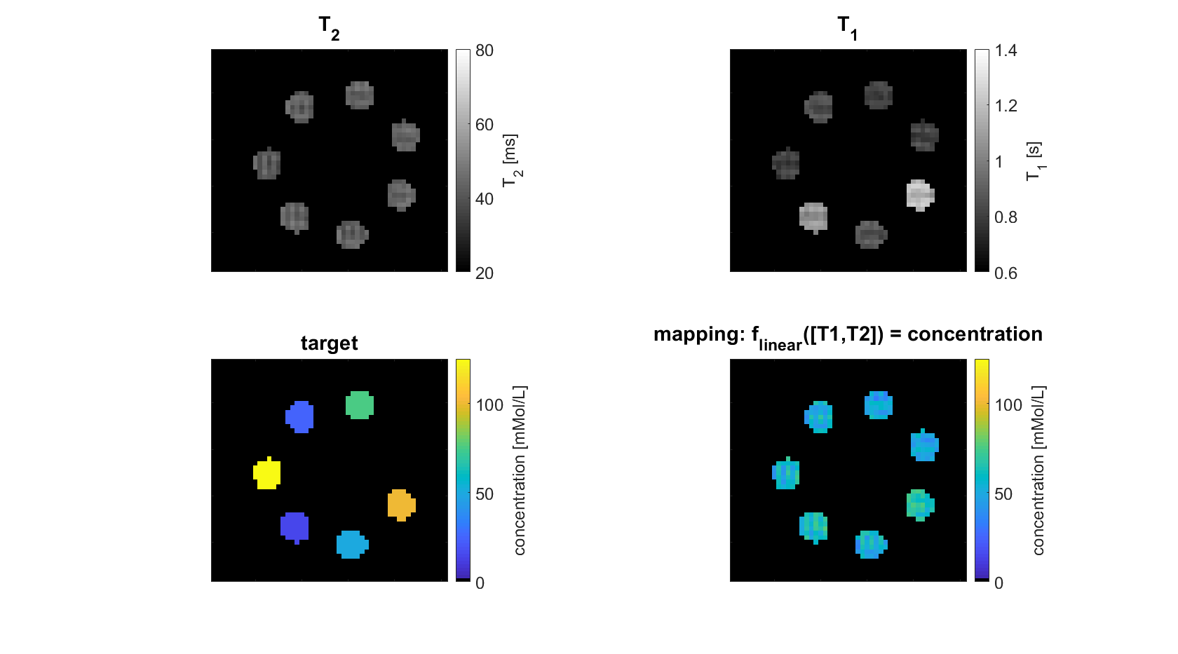
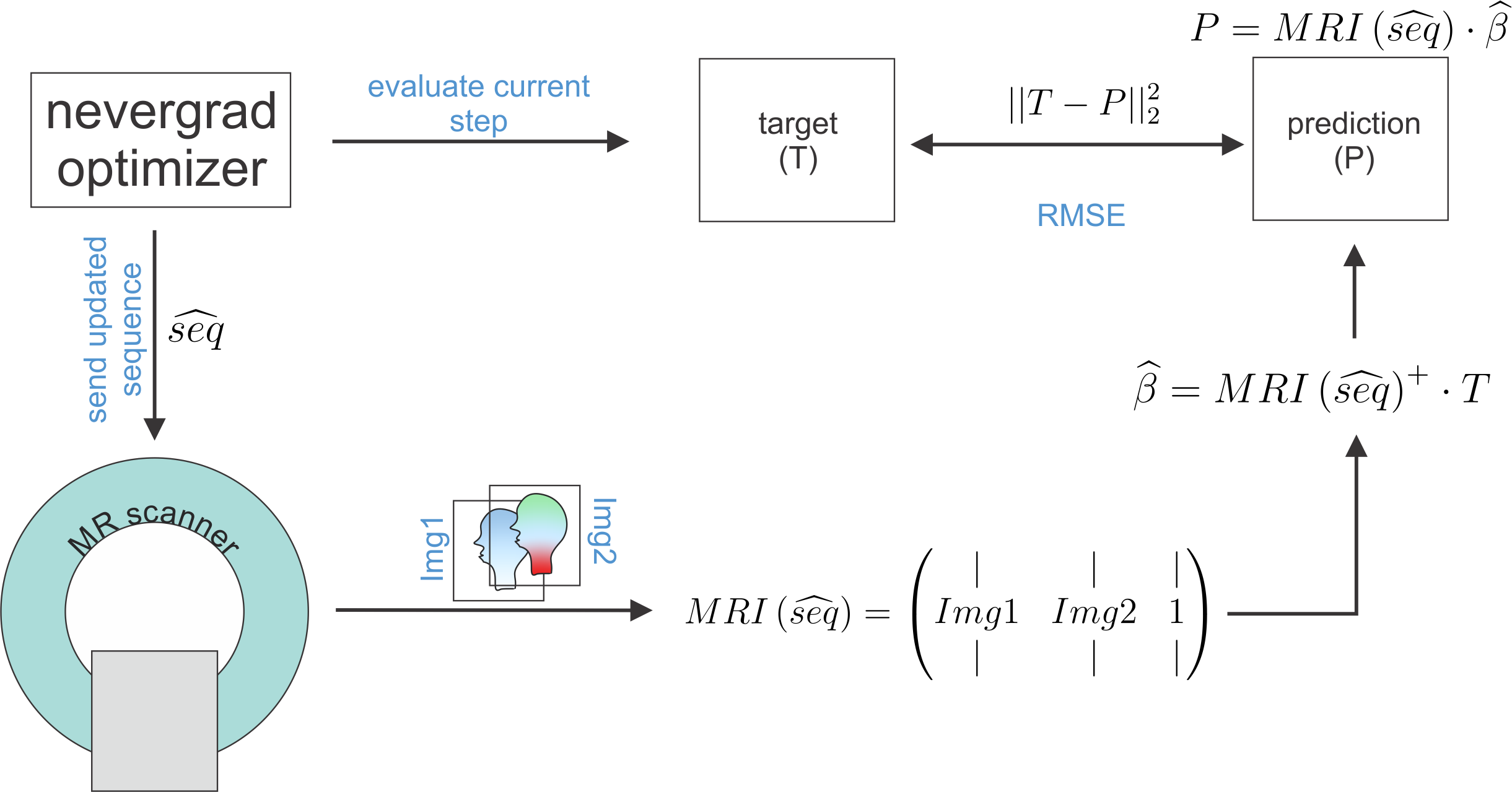
Seven model solutions with different creatine concentration values (0:25:100mMol/L) were created. By adding T1 contrast agent (dotarem®, Guerbet, Germany) and agarose (Carl Roth, Germany) it was made sure that in quantitative T1 and T2 maps obtained from conventional sequences these samples were indiscernible (Figure 1A/B). Starting from an ”empty” RF-prepared sequence with fixed 2D-GRE readout, the CMA-ES optimization algorithm² implemented in nevergrad³ was employed to explore the sequence parameter space including possible RF-preparation events such as number of pulses, amplitude, duration, phase/frequency, and delay times. This type of stochastic optimization algorithm is particularly designed for derivative-free, non-convex, noisy optimization problems as posed by sequence optimization at a real scanner. Every sequence generated by the optimizer is executed directly at the scanner and the intermediate images flow back to the algorithm influencing the next sequence iteration.
For the present work, each sequence iteration consisted of two RF-prepared readouts with the pulse train parameters peak saturation amplitude B_1,1/2, frequency offset $$$\Delta\omega$$$_1/2 and number of pulses np_1/2 as optimized sequence parameters (seq). The reconstructed images IMG(B_1,1,$$$\Delta\omega$$$₁,np₁) and IMG(B_1,2,$$$\Delta\omega$$$₂,np₂) at each iteration were assembled in a design matrix MRI(seq)=[IMG(B_1,1,$$$\Delta\omega$$$₁,np₁);IMG(B_1,2,$$$\Delta\omega$$$₂,np₂);1] of shape #voxels-by-3. Linear regression onto the voxel-wise targets (shape: #voxels–by-1), consisting of known creatine concentrations, was performed by pseudo-inversion of the model $$$T=MRI(seq)\cdot\beta \Rightarrow \widehat{\beta}(seq)=MRI(seq)^{+}\cdot T$$$. The difference between the linear prediction and the true target determined how the optimization algorithm updated the sequence parameters by solving the following non-linear minimization problem:
$$\widehat{seq}=argmin_{seq}\left(||T-MRI(seq)\cdot\widehat{\beta}||_2^2\right)$$
With this problem formulation, the optimizer has to find sequence parameters that yield images that allow the best possible linear mapping to the target contrast (Figure 2). Pulseq⁴ files were used to automatically execute the sequence of each iteration at the scanner. They additionally facilitate numerical simulations of the optimized sequence parameters⁵. Measurements were performed at a 3T PRISMA scanner (Siemens Healthineers, Erlangen, Germany) using the vendor’s 20Ch head coil.

Results

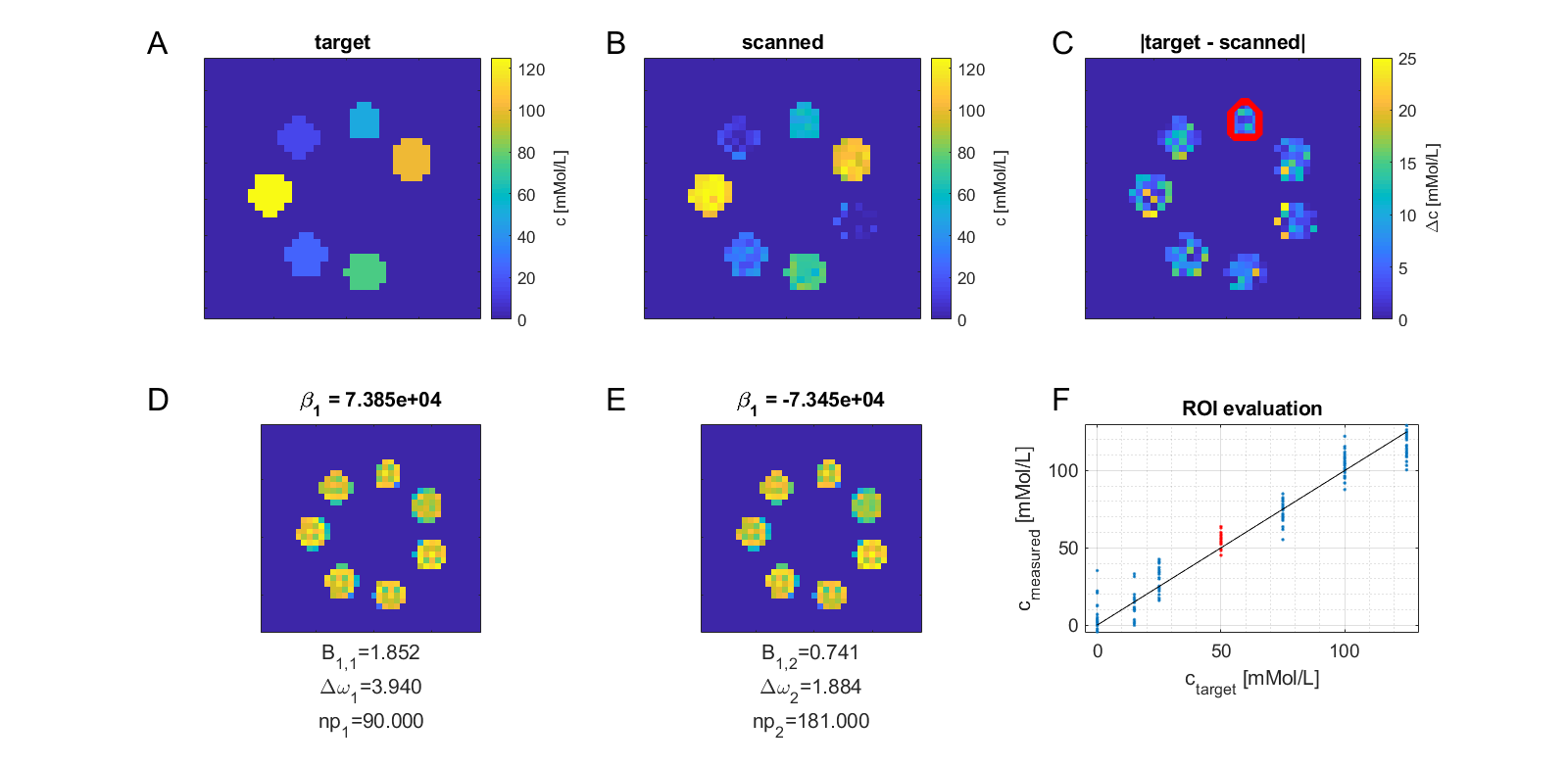
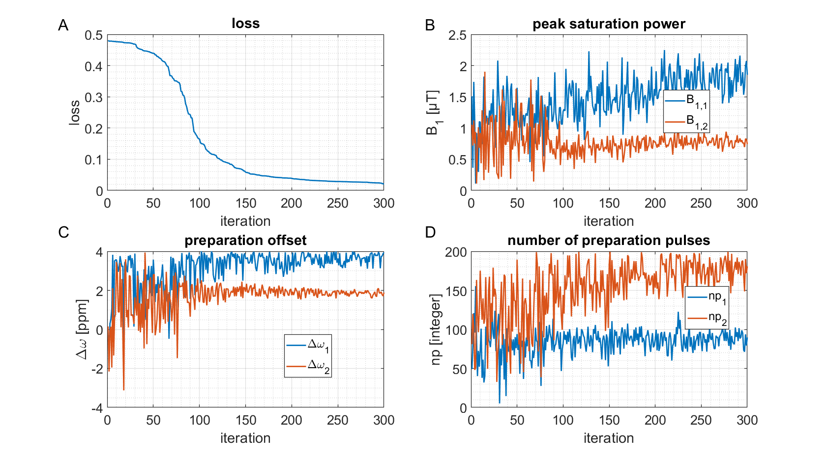
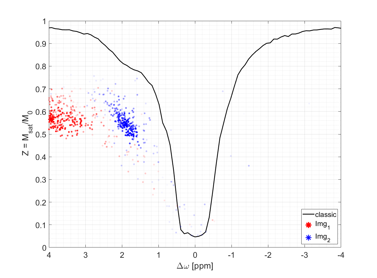
To make sure that the MR-double-zero agent has to find a new sequence concept, and that the creatine concentration cannot be inferred just from T₁- or T₂-weighting, the phantoms were built so that T₁ and T₂ is not governed by creatine proton exchange. This invariance can already be seen in the T₁ and T₂ maps in Figure 1, and was verified by the unsuccessful linear estimation using only T₁ and T₂ as input (Figure 1D). Figure 3B shows the creatine concentration map generated by the newly discovered sequence, which was formed by linear regression from the two RF-prepared images (Figure 3D/E) with optimized sequence parameters. Remarkably, the method generalizes to the vial with 50mMol/L, which was excluded from the ‘training’ procedure, i.e. not considered in the loss function during optimization (Figure 3F). Figure 4 depicts the optimization process of the sequence. An animated version of the optimization can be viewed online (https://owncloud.tuebingen.mpg.de/index.php/s/5nE8mtcRtbHMZww). Learning required 300 iterations, which took around 4h at the MRI scanner. This is long for an MRI scan, but fast for a novel MRI contrast. In contrast to conventional CEST imaging, the optimized sequence required as little as two RF preparation offsets. While in this particular case one of the chosen frequency offsets was at the creatine proton resonance at 1.9ppm, the other one was not chosen at -1.9ppm, but at around 4ppm and with another B₁ amplitude and saturation time (Figure 5). This non-intuitive choice still yielded better results than traditional metric MTRasym⁵.

Discussion

A CEST pool can affect T₁ and T₂ relaxation times, thus adding agar and contrast agent is crucial to make this direct influence negligible and the phantoms undiscernible in conventional contrasts. Still, not T_1w/T_2w, but off-resonant pulses are chosen by MR-double-zero to encode creatine concentration. MR-double-zero can be seen as advanced, sophisticated grid search in the MR parameter space to figure out if a certain contrast can be generated. The optimization problem was reduced to the optimization of as little as three parameters. This is a significantly smaller subset of parameters as compared to the set of parameters required to define an entire MR sequence. The research question is answered based on purely experimental data, relies on a consistent set of phantom properties and thereby includes all possible experimental imperfections

Conclusion

MR-double-zero is able to discover completely new MRI contrasts without requiring an explicit description of the underlying mechanism in form of a theoretical model. This was exemplarily demonstrated for a CEST effect, but it is conceivable that MR-double-zero could also discover yet unknown MRI contrast correlations given suitable phantoms and targets are provided.

Acknowledgements

The financial support of Max Planck Society and German Research Foundation (Reinhart Koselleck project DFG SCHE658/12) is gratefully acknowledged.

References

1.) Loktyushin A, Herz K, Dang N. et al. MRzero —Automated discovery of MRI sequences using supervised learning. Magn Reson Med. 2021;86:709–724.
2.) Hansen N and Ostermeier A; Adapting arbitrary normal mutation distributions in evolution strategies: the covariance matrix adaptation. Proceedings of IEEE International Conference on Evolutionary Computation, doi: 10.1109/ICEC.1996.542381
3.) Rapin J and Teytaud O; Nevergrad - A gradient-free optimization platform. https://GitHub.com/FacebookResearch/Nevergrad
4.) Layton KJ, Kroboth S, Jia F, et al. Pulseq: a rapid and hardware-independent pulse sequence prototyping framework. Magn Reson Med. 2017;77:1544-1552.
5.) Herz K, Mueller S, Perlman O, et al. Pulseq-CEST: Towards multi-site multi-vendor compatibility and reproducibility of CEST experiments using an open-source sequence standard. Magn Reson Med. 2021;00:1–14. https://doi.org/10.1002/mrm.28825
6.) Guivel-Scharen V, Sinnwell T, Wolff SD, Balaban RS. Detection of proton chemical exchange between metabolites and water in biological tissues. J Magn Reson. 1998;133(1):36-45.
7.) Deshmane A, Zaiss M, Lindig T, et al. 3D gradient echo snapshot CEST MRI with low power saturation for clinical studies at 3T. Magn Reson Med. 2018;00:1–12. https://doi. org/10.1002/mrm.27569