Introduction

Lower field MRI systems (<1T) are cheaper, lighter, and less prone to system imperfections than regular 1.5-3T systems [1], which are currently used in clinical practice. The use of balanced steady-state free precession sequences (bSSFP) is an approach to partially compensate for the signal-to-noise ratio (SNR) loss at lower-field systems. In this work, phase-contrast balanced SSFP (PC-bSSFP) [2] was implemented and tested on a clinical MRI system ramped down to 0.75T. Phantom and in-vivo results are compared to a standard 2D spoiled gradient echo phase-contrast sequence (PC-GRE).

Methods

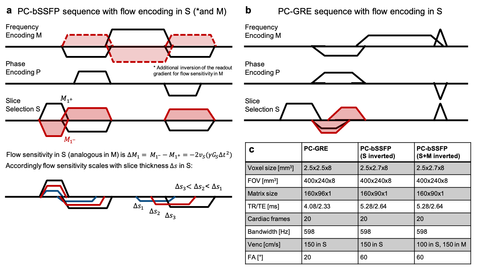
A 3T Philips Achieva scanner was ramped down to a field strength of 0.75T. Using the C13 input channel, proton measurements were performed using a custom-built Helmholtz-like volume transmitter and a four-channel receive coil (Clinical MR Solutions). Flow sensitivity in a 2D bSSFP sequence was achieved by inverting the slice selection gradients between two consecutive scans (Figure1). Flow sensitivity in the slice direction was tuned by adjusting the peak B1 amplitude of the RF pulse. As a reference, a standard PC-GRE sequence with through-plane flow encoding was used. A U-shaped water flow phantom (18 mm diameter) was scanned at velocities of v=0-160 cm/s. Scan parameters for the gated PC-bSSFP and PC-GRE scans are summarized in Figure1. An axial slice perpendicular to the tube axis was chosen, with velocity encoding along the slice-select direction for both scans. An ECG was simulated and, to increase SNR, signals were averaged over all cardiac frames. Concomitant field corrections adapted to 0.75T were performed. Background phase correction and unwrapping was performed on phase difference images of both sequences. A set of coronal PC-bSSFP scans were acquired with the same scan settings. Additionally, to achieve in-plane flow sensitivity in the phantom, coronal scans were acquired with an inverted readout (and slice-select) gradient (Figure1). Cine PC-bSSFP imaging using slice-select gradient inversion was obtained in 6 healthy volunteers (age 30∓2 years) according to institutional and ethical guidelines. PC-GRE scans were acquired alongside and in the same orientation. Scan parameters were the same as for the phantom. Each scan was performed within a breath hold, using ECG triggering and in an axial orientation at the level of the pulmonary arteries, cutting the ascending aorta (AAo) perpendicularly. For axial scans an ROI was drawn in the inflow tube and the AAo. For coronal scans (phantom) an ROI at the level of the axial slice was chosen. As fast flowing water was not fully polarized, a simple inflow model was used to simulate a correction for the phantom data SNR at different velocities, however this does not account for out-of-slice spin history effects.

Results

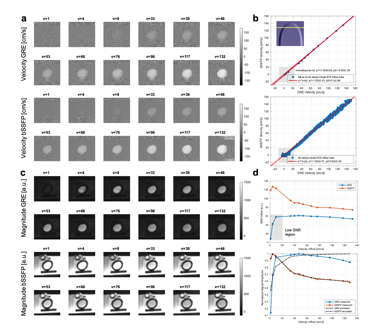
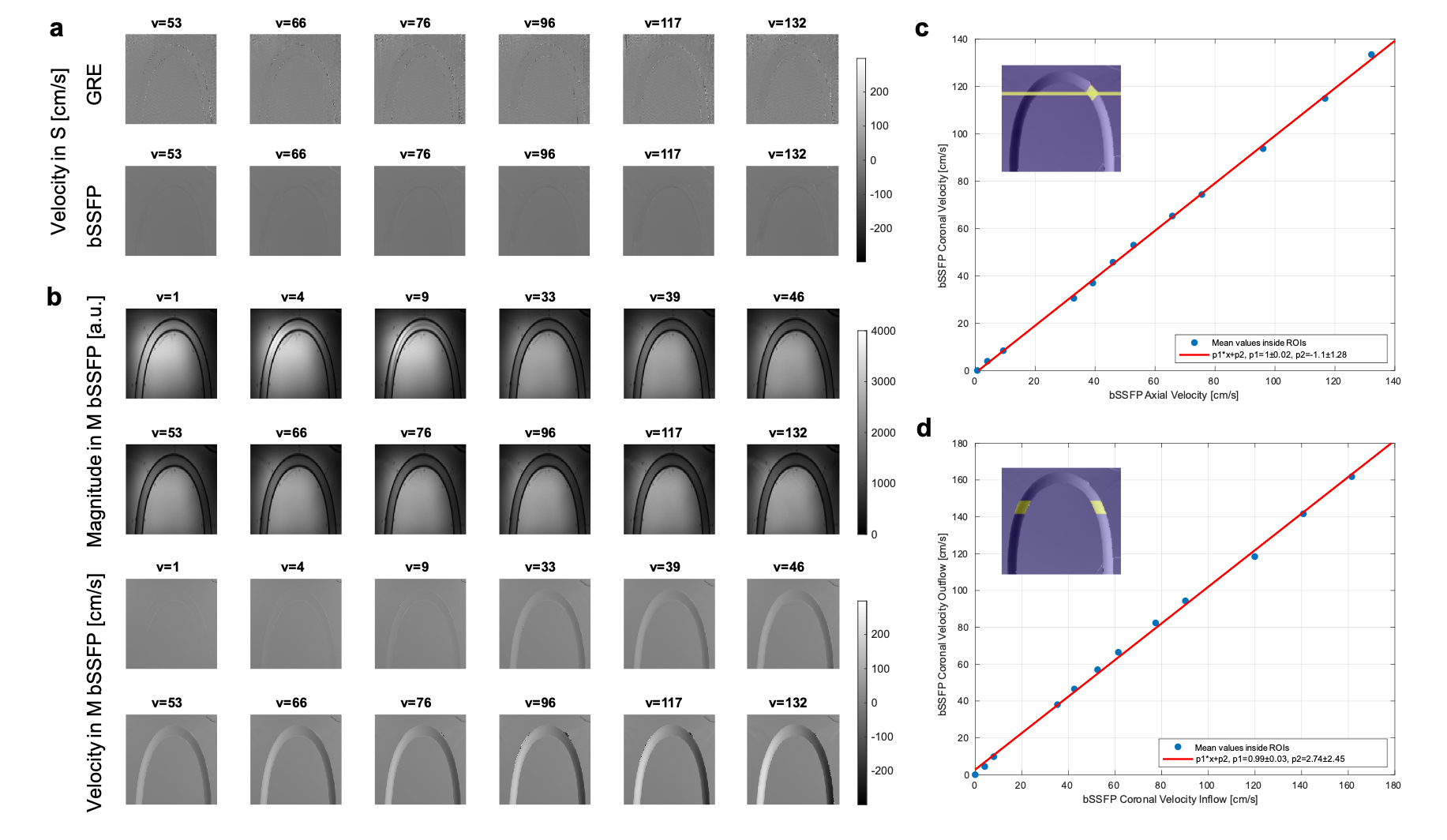
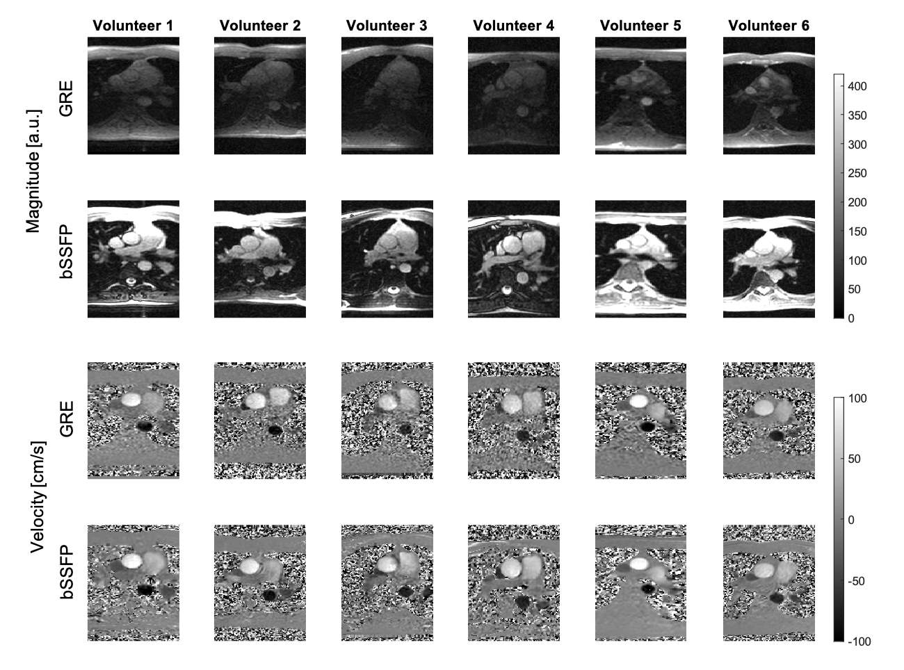
Velocity maps of the axial PC-bSSFP phantom scans (Figure2a) appear less noisy compared to PC-GRE, relating to their higher SNR. The mean velocities inside the ROI showed a good correlation between both sequences at high velocities (slope 1.02∓0.03) (Figure2b). At velocities <20 cm/s PC-GRE started to underestimate velocities by up to 5% due to low SNR. This was also observed when looking at voxel-wise comparisons inside the ROI. Figure 2c shows that the inflow effect in PC-GRE scans led to an increased signal inside the tube at higher velocities, which is also shown in Figure 2d. In contrast, the SNR for PC-bSSFP was always higher than for PC-GRE, but decreased at higher velocities due to inflowing, not fully polarized water. This effect was recreated in simulation. Time-wise averaged phantom results had a sqrt(20)=4.5 times higher SNR than in-vivo scans. No through-plane flow was measured for coronal PC-GRE and PC-bSSFP with velocity encoding in the slice-select direction (Figure3a). This justified PC-bSSFP scans with simultaneous encoding in readout (M) and slice-select (S) direction. Magnitude and velocity images are shown in Figure 3b. Velocities in the coronal scans, encoded in M, compared well to axial images, encoded in S (slope 1.00∓0.02). Also in- and outflow velocities inside the coronal slice compared well (slope 0.99∓0.3) (Figure3c-d). In-vivo axial PC-bSSFP showed higher signal in the magnitude and less noise in the velocities when compared to PC-GRE (Figure4). Both sequences were able to capture time-resolved flow and anatomical information at 0.75T. Velocity curves in the AAo for all volunteers agreed well for both sequences, whereas the SNR in PC-bSSFP scans was on average 2-3 times higher when compared to PC-GRE scans (Figure5a-b). The SNR in PC-GRE also showed a strong dependency on the velocities within the cardiac cycle, whereas the PC-bSSFP SNR was stable over time. Comparison of velocities in the AAo (Figure5c) showed a good correlation between the methods (slope 1.01∓0.03) with a slight (0.48∓4.38 cm/s) underestimation of PC-GRE velocities.

Discussion

The velocity-to-noise ratio is proportional to the signal SNR, which is why SNR-efficient sequences such as bSSFP become important at lower field strengths. In this study PC-bSSFP and PC-GRE velocity values compared well, demonstrating the value of PC-bSSFP sequences at lower field strengths. The challenge of PC-bSSFP imaging remains flow and offset frequency dependent artefacts, which however also decrease with field strength.

Conclusion

We have demonstrated the feasibility and accuracy of cine phase-contrast bSSFP flow measurements at a lower field MRI system.

Acknowledgements

No acknowledgement found.