0082
Automatic background phase correction on 4D Flow using M-estimate SAmple Consensus (MSAC)1Department of Medical Imaging, Technical University of Berlin, Berlin, Germany, 2Magnetic Resonance, Siemens Healthcare GmbH, Erlangen, Germany, 3Physikalisch-Technische-Bundesanstalt (PTB), Braunschweig and Berlin, Germany, 4School of Imaging Sciences and Biomedical Engineering, King's College London, London, SE1 7EH, United Kingdom, 5Institute of Radiology, University Hospital Erlangen, Friedrich-Alexander-Universität Erlangen-Nürnberg (FAU), Erlangen, Germany
Synopsis
4D Flow data requires background phase removal to correctly quantify flow velocities. Typical methods are semi-automatic, requiring manual parameter input and remain time-consuming. Furthermore, correction methods based on stationary tissue segmentation fail when in the presence of wrap-around artifacts. In contrast, the proposed M-Estimate SAmple Consensus (MSAC) algorithm robustly and fully automatically corrects background phases by rejecting pixels that show large deviations from the most probable phase offset fit. A parameter sensitivity analysis is proposed following in vivo application in 13 datasets.
Introduction
4D Flow is a valuable tool to derive a wide range of hemodynamic parameters. However, background phase offsets, mainly generated by eddy currents, often hamper their clinical confidence and acceptance1. A typical correction strategy consists of semi-automatically segmenting stationary tissue and performing a nth-order polynomial fit on the phase data2. Additionally, to requiring user input, this method typically fails in presence of wrap-around artifacts3. Recently, an outlier detection algorithm to discard wrap-around was proposed5-6, which assumes that the central 50% of the FOV are without wrap-around.We previously introduced and analyzed the performance of M-estimate SAmple Consensus7 (MSAC) on 2D flow imaging8. In this work, we optimize the method for 4D Flow, analyze its robustness to algorithm parameters and investigate its performance with and without wrap-around by comparing it to stationary tissue fit corrections.
Methods
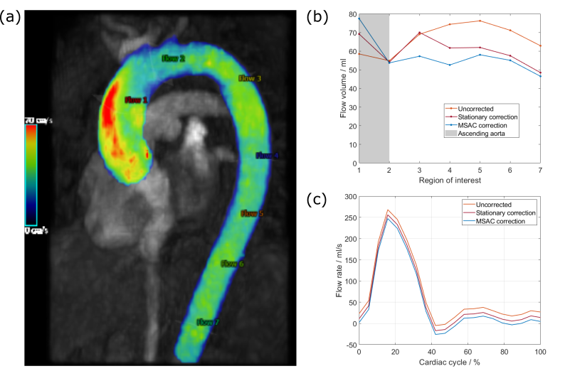
Acquisition:21 4D Flow datasets of the aortic arch with varying degrees of wrap-around (Figure 1a-b) were acquired in eleven volunteers on two MRI systems (MAGNETOM Sola/Vida, Siemens Healthcare, Erlangen, Germany) using multi-channel body and spine coil arrays. A retrospectively ECG and prospective breathing navigator-gated, velocity-encoded (venc=150cm/s), spoiled gradient-echo sequence was used. As a ground-truth correction, acquisitions were repeated on stationary phantoms following each volunteer.
Correction:
For MSAC correction, a mask using the temporally averaged magnitude image was created (pixel pool M). From the phase volume, MSAC then randomly selects m samples from M on which it fits a 3D polynomial. Outliers are selected based on the absolute distance $$$\epsilon$$$ of pixels in the pool M and on the fitted volume. Pixels below a threshold $$$t$$$ build a consensus set. This selection and fitting process is repeated N times (Fig1c).
After all iterations, the consensus set $$$C_n$$$ with lowest cost
$$C_n = \sum_{i\in\mathrm{M}}\left\{\begin{matrix}\epsilon_i&\epsilon_i<t,&\\t&\epsilon_i\ge t&\end{matrix}\right.$$
is selected and all included pixels are used for the final background fit.
Each phase (velocity) volume is processed independently.
An analysis of MSAC parameters and fit orders was performed on 8 acquisitions from both field strengths.
Following this sensitivity analysis, MSAC parameters were set to N=30, m=10 and t=0.015*venc. MSAC pixel selection was based on a 1st-order polynomial while a 3rd-order polynomial background fit correction was performed on the remaining 13 datasets.
MSAC was compared to phantom correction and 3rd-order stationary tissue fit correction, which describes a mask based on the thresholded temporal variance of the phase volume2.
Evaluation:
Fit quality was assessed by the root-mean-squared error (RMSE) between background fit and phantom measurements in pixels p within a sphere-shaped ROI (50mm radius placed in the center of the phantom)
$$\mathrm{RMSE}_j=\sqrt{{1}/{\mathrm{N}_\mathrm{ROI}}\sum_{i\in N_\mathrm{ROI}}\left(p_{i,j}-p_{i,j,\mathrm{Phantom}}\right)^2}$$
The RMSE is calculated individually for each velocity encoding direction $$$j$$$.
Additionally, flow volumes between a stationary fit and MSAC corrected image were compared in the ascending and descending aorta.
Flow analysis was performed using cvi429. Computations were performed in Matlab10.
Results
Figure 2 shows example masks generated by MSAC and the stationary fit correction for an image with wrap-around highlighting areas in which MSAC successfully ignores areas of wrap-around.Figure 3a-c demonstrates robustness for large ranges of MSAC parameters when assuring a minimum number of iterations (N=10) and avoiding very low or very high threshold values.
The accuracy as a function of spatial order (Figure 3d-f) demonstrates that MSAC performs best with 1st-order detection followed by a 3rd-order correction.
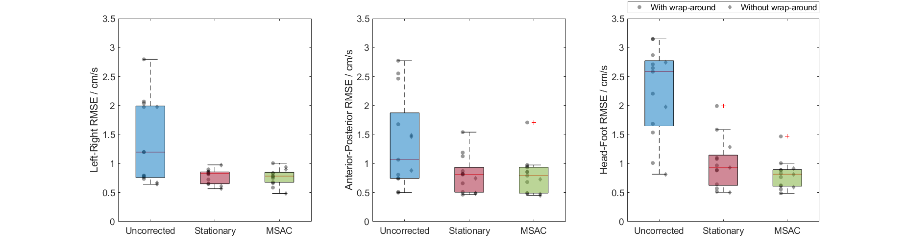
Figure 4 compares uncorrected, MSAC- and stationary tissue correction over all acquisitions. In left-right direction, the median drops from 0.82cm/s to 0.78cm/s, while the range slightly increases from (0.64-0.98)cm/s to (0.48-1.01)cm/s. Anterior-posterior, the median and range drop from 0.81cm/s (0.46-1.54)cm/s to 0.79cm/s (0.45-0.98)cm/s and in head-foot direction, both drop from 0.93cm/s (0.51-1.6)cm/s to 0.81cm/s (0.49-1.01)cm/s.
MSAC takes 1.01±0.04s on average.
An exemplary flow volume analysis is depicted in Figure 5.
Discussion
MSAC successfully optimizes the number of inliers with respect to their residuals across the entire image which is why only the tissue that does not fit is rejected. Non-fitting tissue is mostly, but not only in the wrap-around area of the image and includes flow-regions as well (Figure 2).Although MSAC shows dependencies on its parameters (threshold, number of trials, fit orders), the study showed that a universal set of parameters is applicable to all dataset and both field strengths.
As expected, stationary tissue correction in 4D Flow performs better than in 2D Flow5,8 due to increased availability of credible pixels. This lead to comparably less, however improvement when using MSAC as compared to stationary tissue correction (Figure 4). MSAC clearly reduces the spread of RMSE after correction. As expected, MSAC performed well, independently of field strength.
The presented in vivo case (Figure 5) shows that different masks can still lead to different correction results, since minor differences in flow rates result in larger deviations of flow volumes.
Conclusion
We showed that MSAC can be applied to 4D Flow and robustly corrects for background phases. A fixed set of parameters can be used making MSAC a fully automatic correction, easily integrable into clinical workflow. Initial in-vivo flow quantification demonstrated its successful integration. Further investigation includes the comparison to other methods3-5, its in-line integration on the scanner and its application in patients.Acknowledgements
No acknowledgement found.References
[1] Gatehouse P, Rolf M, Graves M, et al. Flow measurement by cardiovascular magnetic resonance: A multi-centre multi-vendor study of background phase offset errors that can compromise the accuracy of derived regurgitant or shunt flow measurements. J Cardiovasc Magn Reson. 2010;12(1):1-8. doi:10.1186/1532-429X-12-5
[2] Walker PG, Cranney GB, Scheidegger MB, Waseleski G, Pohost GM, Yoganathan AP. Semiautomated method for noise reduction and background phase error correction in MR phase velocity data. J Magn Reson Imaging. 1993;3(3):521-530. doi:10.1002/jmri.1880030315
[3] Gatehouse PD, Rolf MP, Bloch KM, et al. A multi-center inter-manufacturer study of the temporal stability of phase-contrast velocity mapping background offset errors. J Cardiovasc Magn Reson. 2012;14(1):1-7. doi:10.1186/1532-429X-14-72
[4] Ebbers T, Haraldsson H, Dyverfeldt P, Sigfridsson A, Warntjes M, Wigström L. Higher order weighted least-squares phase offset correction for improved accuracy in phase-contrast MRI. In: Proc. Intl. Soc. Mag. Reson. Med. ; 2008.
[5] Pruitt, A. A., Jin, N., Liu, Y., Simonetti, O. P., & Ahmad, R. (2019). A method to correct background phase offset for phase-contrast MRI in the presence of steady flow and spatial wrap-around artifact. MRM, 81(4), 2424–2438. doi:10.1002/mrm.27572
[6] Pruitt AA, Jin N, Liu Y, Simonetti O, Ahmad R. Background phase correction in the presence wrap-around artifact : Application in 4D Flow imaging. In: Proc. Intl. Soc. Mag. Reson. Med. ; 2018.
[7] Torr PHS, Zisserman A. MLESAC: A new robust estimator with application to estimating image geometry. Comput Vis Image Underst. 2000;78(1):138-156. doi:10.1006/cviu.1999.0832
[8] Fischer C, Wetzl J, Schäffter T, Giese D. Automatic and robust background phase correction on phase-contrast MRI using M-estimate SAmple Consensus (MSAC). In: Proc. Intl. Soc. Mag. Reson. Med. ; 2021.
[9] Circle Cardiovascular Imaging, Inc. : cvi42(Release 5.13.7 (2335)) [Computer Software].
[10] The MathWorks, Inc. (2018). Matlab (Version R2019b) [Computer Software]. https://mathworks.com/
Figures
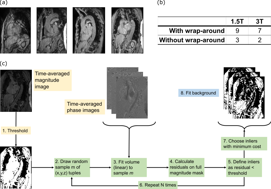
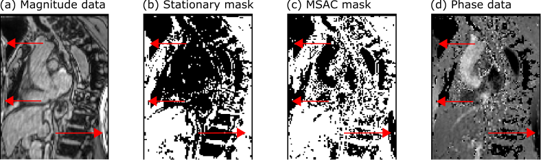
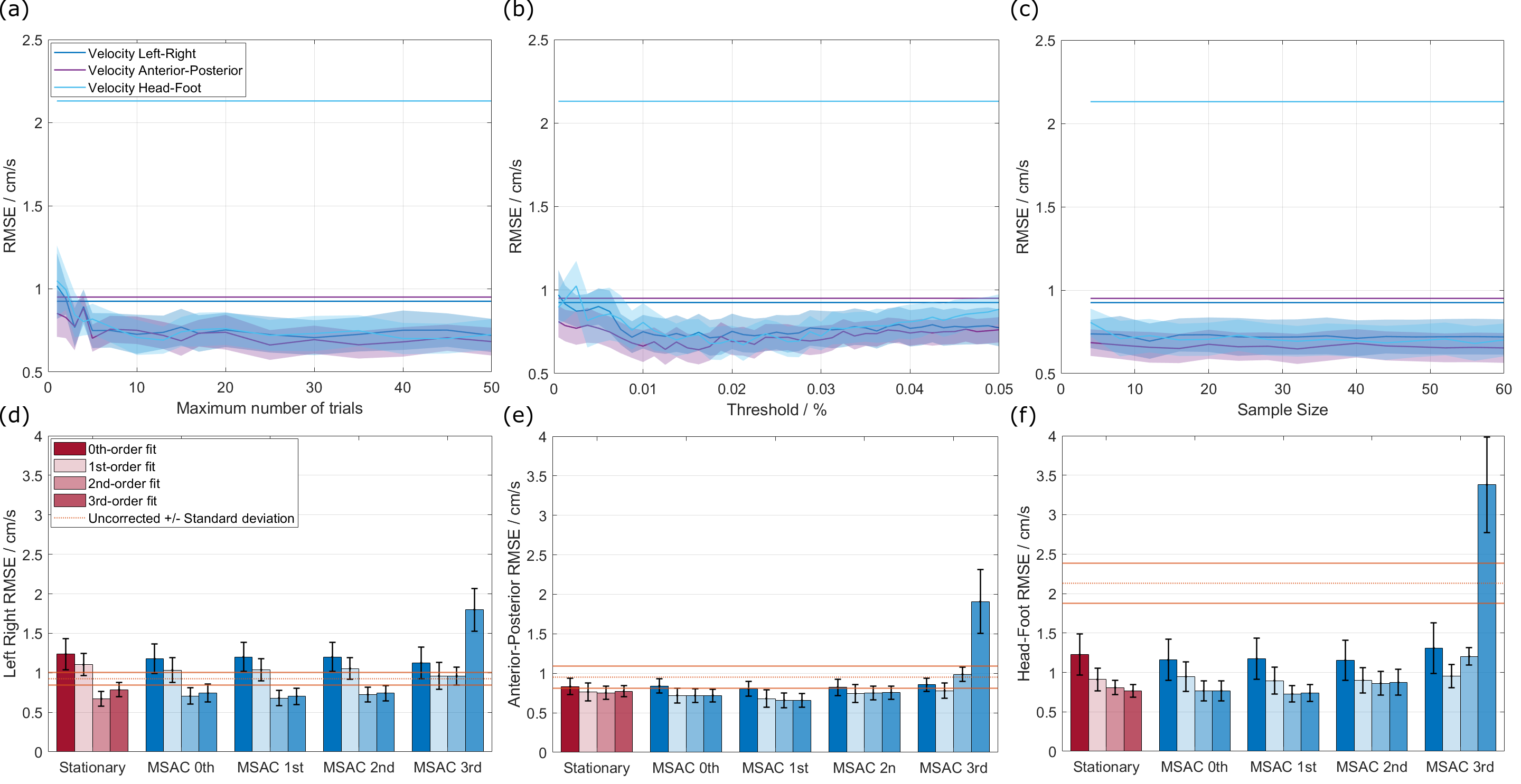
Figure 3: (a)-(c): Sweep over different values for number of trials (a), threshold (b) and sample size (c). All encoding directions are plotted and compared to corresponding uncorrected background offsets (straight line).
(d)-(f): For all encoding directions, different polynomial fit orders during MSAC selection are compared to stationary correction. Additionally, the final correction fit order is varied (opacity). Differences are small between 0th-, 1st- and 2nd-order selection .