0063
A New Approach to Shimming Halbach Arrays Using Higher Order Halbach Array Inserts1Radiology, Leiden University Medical Center, Leiden, Netherlands
Synopsis
Halbach arrays are an appealing magnet design for low field MRI due to their low weight and cost typically suffer from relatively high B0 inhomogeneity. In this work we show a new approach to shimming Halbach arrays using higher order Halbach inserts which can be designed to target specific spherical harmonic terms. We demonstrate the principle by correcting for the x2-y2 spherical harmonic, improving B0 homogeneity of a 31cm diameter bore Halbach array by 50% and show that in simulations homogeneities of 280 ppm can be achieved over a 20 cm sphere by correcting up to 5th order spherical harmonics.
Introduction
Halbach arrays are an appealing approach for low field MRI due to low cost and weight [1,2] but typically suffer from poor B0 homogeneity. B0 imperfections can be introduced by variations in the magnetization strength and direction of the individual magnets[3] or manufacturing tolerances in the magnet formers. Arrays typically need several shimming iterations, involving the addition of magnetic material inside the magnet, with positioning often calculated using stochastic algorithms.We present a new shimming approach that exploits the field patterns created by higher-order Halbach shim-arrays to correct for distinct spherical harmonic B0-inhomogeneity terms. A homogenous B0 field (degree (l) = 0, order (m) = 0 spherical harmonic) is generated using a cylindrical dipolar (k=1) Halbach array where the magnetization direction rotates twice over circumference of the cylinder. A transverse linear gradient (l=1, m=|1| spherical harmonics) can be created using a quadrupolar (k=2) (see figure 1) Halbach array comprising three rotations over the surface, etc. For spherical harmonics where l > m, the field can be approximated by varying the magnetization of the Halbach array along its length. For example, to create a linear gradient along the bore (l=1, m=0) one could use a k=1 Halbach array with the sign of the magnetization reversing (smoothly) along its length. As such, given a sufficiently long Halbach array, a k=1 shim can be used to generate all spherical harmonics of order 0. We demonstrate this concept on a new custom-built 47 mT, head system where we improve the homogeneity of the magnet by 50% by only correcting for the m=2 spherical harmonics.
Method
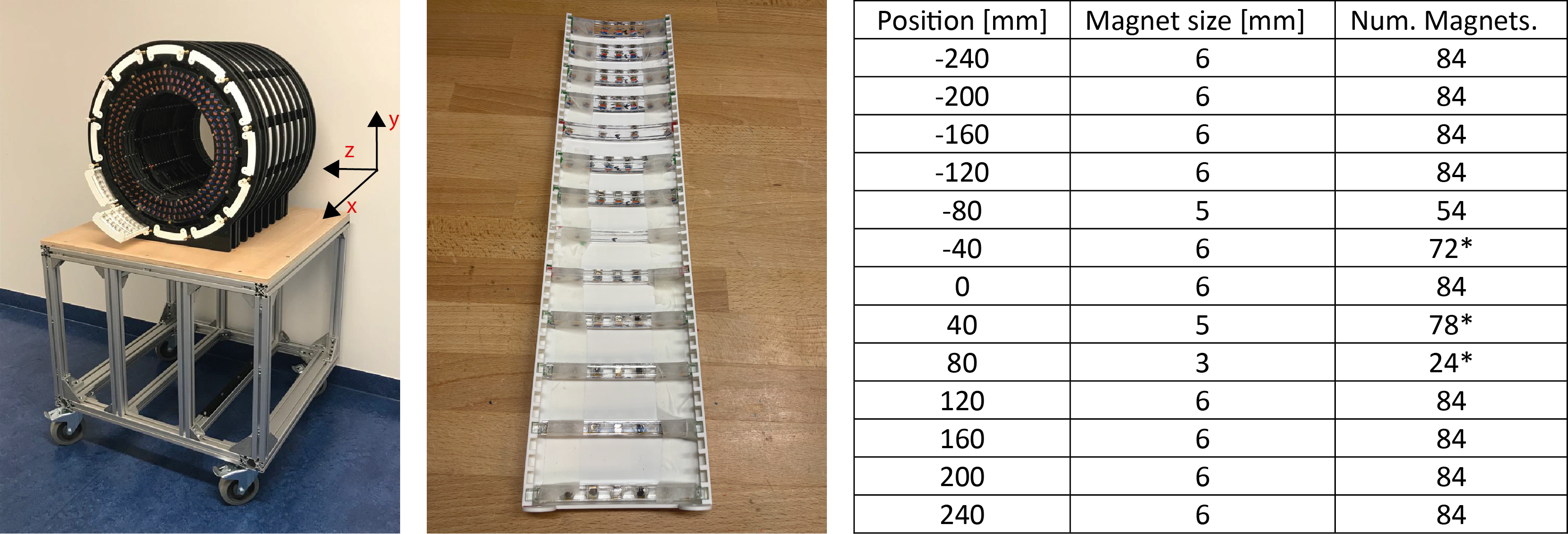
A 50 cm long, 31 cm diameter bore Halbach array based magnet was designed using the variable diameter homogeneity optimisation described previously [6]. The magnet consists of 25 rings, with 20 mm centre-to-centre spacing, of 12 mm cuboid N48 magnets: the central 19 rings have two layers of magnets and the three rings at each end have 3 layers. The magnetic field was mapped over a 250 mm diameter spherical volume (DSV) with a Teslameter attached to a 3D positioning robot. The acquired field maps were fitted to up to 20th order spherical harmonics to reduce noise. The inhomogeneity over a 25 cm DSV was measured to be 11723 ppm (figure 3). The l=2 , m=2 spherical harmonic term was the most significant contributor with a magnitude of 10245 ppm and as such we designed a k=3 Halbach shim array.Shim magnets (up to 6 mm) are placed in 12 holders located on the outside of the magnet (see figure 2): each holder can accommodate 49 trays of magnets with 10 mm spacing between the trays. For the first shim iteration we filled only 13 trays (40 mm spacing) to allow for later iterations. Magnets were placed on a cylindrical radius with up to seven magnets per tray segment (84 in total for each position along the magnet). The field distribution generated by each ring of magnets was calculated, and a least squares fit of the field performed to calculate the total magnetization needed in each ring. This was then approximated by varying the size and number of magnets in each ring. An experimental field map was acquired after shimming and we simulated a correction of up to 5th order spherical harmonics based on this map.
To show the impact of the shim insert, spectra and images of an 8 centimeter spherical phantom were acquired. In both cases the field was shimmed using the linear gradients prior to data acquisition. Images were acquired using a 3D TSE sequence with the following scan parameters: FoV: 150x150x150 mm, resolution: 1.5x1.5x1.5 mm, TR/TE: 600ms/15ms, ETL: 20, bandwidth: 20kHz, duration: 5 minutes
Results
Figure 2c shows the magnet configuration after optimisation with a single populated shim tray shown in 2b. The initial field (figure 3) shows the characteristic Z2 – Y2 spherical harmonic field. The correction field created by a k=2 Halbach shim array closely matches this inhomogeneity. There is good agreement between the simulated (6156 ppm) and measured (5879 ppm) fields after shimming. Simulations of corrections show the B0 homogeneity can be improved to 2771 ppm using shim arrays up to k=6 with only high frequency perturbations at the outer bore remaining. Over a 20 cm DSV, sufficient for full brain coverage, homogeneity improves to 282 ppm using the same correction. Figure 5 shows that the acquired spectra and images are significantly improved after the shims are inserted.Discussion
In this work we show a new approach to shimming Halbach-array magnets using higher order Halbach shim arrays to correct for spherical harmonic inhomogeneities. We achieve a 50 % reduction in inhomogeneity by correcting only for the m=2 order, with excellent agreement between simulations and measurements, showing promise for using this approach for correcting a larger set of spherical harmonics. There are practical limits to the highest order spherical harmonics one can correct due to discretization errors associated with the very high number of rotations needed. While we have applied this method to shimming an existing magnetic field, the basic principle could also be used to optimize the field distribution of new magnets designs.Acknowledgements
This work is supported by ERC Advanced Grant PASMAR and Simon Stevin Meester AwardReferences
[1] Cooley C. et al. A portable scanner for magnetic resonance imaging of the brain. Nat. Biomed. Eng. 2020
[2] O’Reilly T et al. In vivo 3D brain and extremity MRI at 50 mT using a permanent magnet Halbach array. Magn. Reson. Med. 2020;85:495-505
[3] Hugon C et al. Design of arbitrarily homogeneous permanent magnet systems for NMR and MRI: Theory and experimental developments of a simple portable magnet. J. Magn Reson. 2010;205:75-85
[4] O’Reilly T, A. Webb. The role of non-random magnet rotations on main field homogeneity of permanent magnet assemblies. Proc Intl Soc Mag Reson Med (2021) 4042.
[5] Blümler P. Proposal for a permanent magnet system with a constant gradient mechanically adjustable in direction and strength. Concepts Magn Reson Part B Magn Reson Eng. 2016; 46(1);41-48
[6] O’Reilly et al. Three-dimensional MRI in a homogenous 27 cm diameter bore Halbach array magnet. J. Magn Reason. 2019; 307; 106578
Figures
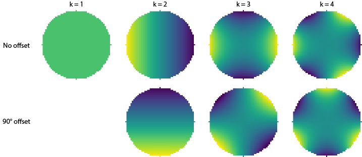
Transverse views of magnetic field patterns created by cylindrical Halbach arrays of different orders: in the bottom row the magnet rotations are offset by 90 degrees. The field patterns correspond to spherical harmonics of order m = 0 for k=1 up to m = |3| for k = 4, where the 90 degree offset changes the sign of the order (i.e. for k = 3 with no offset the field corresponds to the l = 2, m = 2 spherical harmonic, and with a 90 degree offset to l = 2, m = -2).
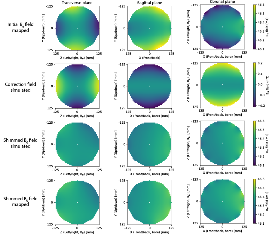
1st row) Initial B0 field map shown in three planes of the 25 cm diameter spherical volume. Inhomogeneities in the transverse plane are dominated by the 2nd order Z2 – Y2 spherical harmonic term. 2nd row) The simulated shim field created by a k=3 (quadrupolar) Halbach shim insert. 3rd row) Simulated B0 field map after applying the shims. 4th row) The measured field map after the shims are placed, showing excellent agreement with simulations. The initial inhomogeneity over a 25 cm sphere was 11723 ppm, the simulated shimmed field was 6156 ppm and the measured field after shimming was 5879 ppm.
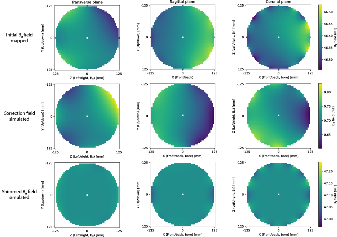
Figure 4. Simulations of the shimming performance when correcting for up to m=5 shims. The initial inhomogeneity over a 25 cm DSV is 5879 ppm which is decreased to 2771 ppm after shimming. The remaining perturbations have a relatively high spatial frequency which may be difficult to correct with shim trays placed on the outside of the magnet and may require the placement of magnetic material on the inside of the magnet.
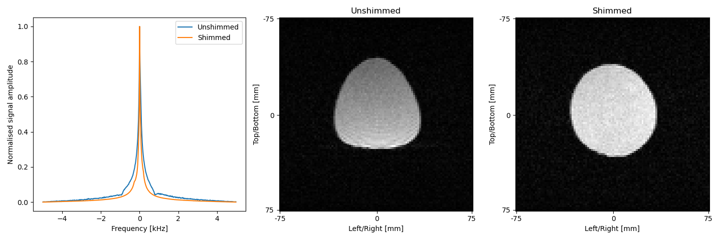
Left) Spectra acquired of an 8cm spherical phantom with an without the shim inserts added. Middle and right) Images acquired using a TSE sequence of the same ball phantom. In all cases additional shimming was performed using the gradient coils. The line width and the image distortions are substantially improved after the shims are added to the system.