4301
Connectoflow: A cutting-edge Nextflow pipeline for structural connectomics1Electrical Engineering, Vanderbilt University, Nashville, TN, United States, 2Computer Sciences, Université de Sherbrooke, Sherbrooke, QC, Canada, 3Faculté de médecine et des sciences de la santé, Université de Sherbrooke, Sherbrooke, QC, Canada, 4Centre de Recherche du Centre Hospitalier, Université de Montréal, Montréal, QC, Canada, 5Department of Neurology and Neurosurgery, McGill University, Montréal, QC, Canada, 6Computer Science, University of Verona, Verona, Italy
Synopsis
Tractography involves complicated processing and connectomics include even more complexity. To facilitate structural connectome reconstruction we present: Connectoflow. Connectoflow requires simple inputs, has simple options and provides simple outputs, all with cutting-edge processing. By leveraging the simplicity of Nextflow and Docker/Singularity, Connectoflow is robust and efficient. By combining Tractoflow with Connectoflow, one can go from raw DW-images to structural connectomes in a few simplified steps. The proposed pipeline innovates by including connection-wise cleaning/filtering, provides connection weights that go beyond streamline count (COMMIT) as well as advanced connection-wise metrics (similarity and AFD).
Introduction
DMRI is the tool of choice to probe structural connectivity. Tractography attempts to reconstruct pathways interconnecting the various regions of the brain [1,2,3], which can be investigated using connectomics [4,5,6,7]. The final output of connectomics is often presented in the form of connectivity matrices that report values for each pair of cortical parcels. The reported values are often, but not limited to, streamline-count, average fractional anisotropy (FA) or volume. Most structural connectivity pipelines go directly from tractogram to these connectivity matrices without much consideration and processing, hiding or ignoring certain steps that may be crucial in producing high-quality connectomes.Tractography is famously complex to process. It requires a sequence of steps that are not trivial. Various pipelines were proposed to facilitate tractography and bridge the gap with the clinical world. Tractoflow [8] was recently proposed as a solution to have cutting-edge processing, efficient, reproducible and easy-to-use by leveraging nextflow [9] and the best tools from various groups [10,11,12]. Connectoflow goes in the same direction, it innovates by incorporating a connection-wise cleaning approach, provides connection-weights that go beyond streamline-count as well as cutting-edge connection-wise (fixel, similarity) measures.
Methods
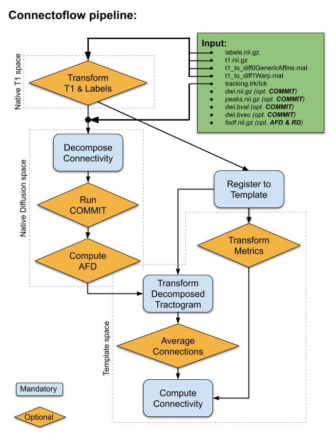
The pipeline was designed to allow for the simplest inputs possible, but to include advanced processing (see Fig. 1). The key steps in Connectoflow are:- Decompose: This step performs the parcel-to-parcel decomposition of the tractogram. It includes streamline-cutting operations [13] to maximize the number of streamlines with terminations in the provided atlas. Moreover, connection-wise cleaning processes that remove loops, discard spurious streamlines and discard incoherent curvatures are used to remove as many false positives as possible [13].
- COMMIT: To further decrease the number of invalid streamlines and assign a quantitative weight to each streamline, Convex Optimization Modeling for Micro-structure Informed Tractography (COMMIT) [14,15] is used. This not only allows the removal of aberrant/spurious streamlines, but it was shown to increase reproducibility of connectivity measures by being more robust to various tractography biases.
- AFD: Apparent Fiber Density (AFD) [16,17] is subsequently computed connection-wise using streamline orientations (fixel), which can be computationally burdensome if done on every pairwise connection of the connectome a posteriori. This step will provide a AFD-weighted connectivity matrix.
- Similarity: The last key step was designed to further reduce risk of false-positives, at the connection level (not at the streamline level). To achieve this, all tractograms are co-registered to a template, each connection is used to compute a population-average connection that represents its overall shape. This population-average is then used to compute a distance between corresponding connections across subjects [18,19]. This distance (mm) is indicative of the similarity to the population to identify connection of interest (small distance) or discard aberrant connection (high distance). This step will provide a similarity-weighted connectivity matrix.
Further connectivity/connectomics scripts are also available through Scilpy (https://github.com/scilus/scilpy) to manipulate, filter, visualize, compute graph measures and perform basic statistics with matrices.
Results
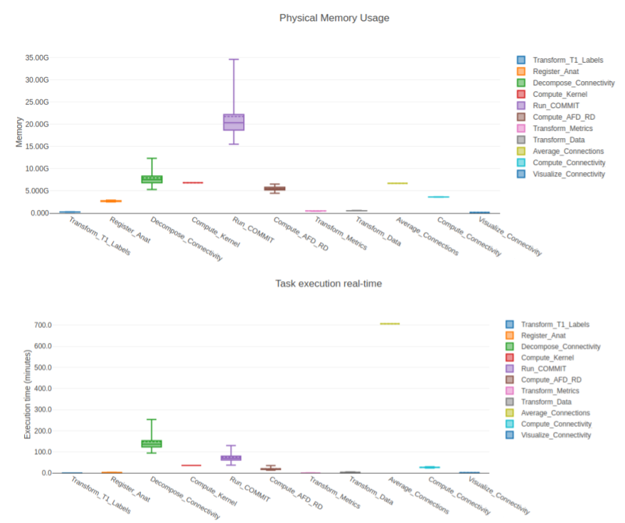
To showcase our pipeline, we processed 105 subjects from the HCP [20] and 230 subjects from the UKBioBank [21]. Tractograms were produced using Tractoflow and parcellations using Freesurfer Desikan-Killiany [22] (an in-house pipeline was made to easily produce Brainnetome [23] and Glasser [24]). In this work, we simply report computational results of the pipeline (see Fig. 4).Tractography was generated using 30 seeds per voxel in the WM for local probabilistic tracking and 100 seed per voxel in the WM/GM interface for particle filtering tracking [24] the HCP data in its native resolution (1.25mm isotropic) and 10 seed per voxel in the WM for local probabilistic tracking and 30 seed per voxel in the WM/GM interface for particle filtering tracking for the UKBioBank in 1.0mm isotropic.
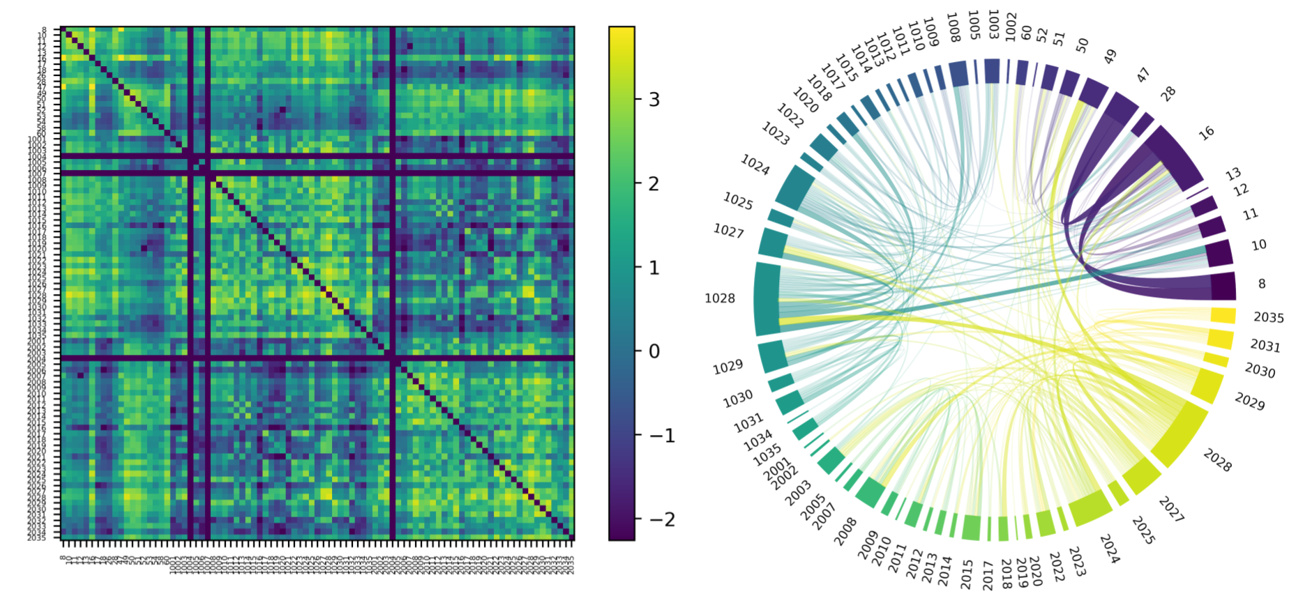
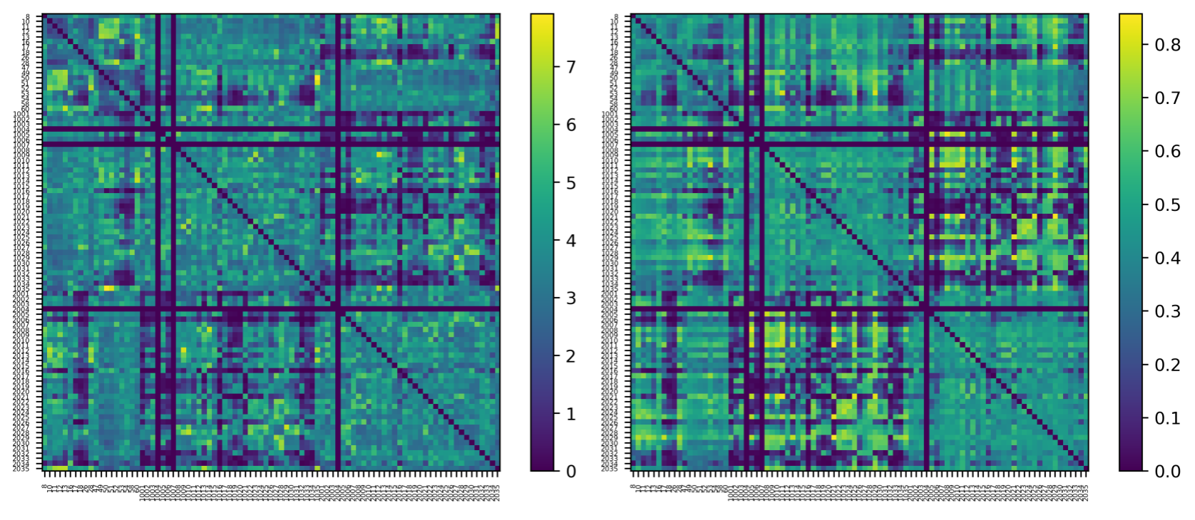
Figures 2 and 3 show examples of the final output of the average connectivity matrix across the UKBioBank dataset. Parcels are ordered as increasing values in the lookup-table. A lot more weighting options are available, this is only a relevant subset to showcase key steps described earlier.
Discussion
The main quality of Connectoflow ease of use. The steps described earlier are difficult to put in place, even for an experienced programmer. Connectoflow allows to simplify processing from tractograms to connectivity matrices. The current, available online, version (https://github.com/scilus/connectoflow) is even simpler to use and even more so when in conjunction with Tractoflow (https://github.com/scilus/tractoflow). Overall, Connectoflow is more efficient for the computer and less time consuming for the user, while providing cutting-edge steps.An important observation for Connectoflow is that the size of the input tractogram will not only impact the processing time, but the memory usage. Both will have to be considered when launching the pipeline on processing clusters or personal computers. Since some of our advanced processing steps are connection-wise (decomposition, AFD or similarity), the number of parcels (hence, the number of connections N^2) will have a large effect on computing time.
Conclusion
Connectoflow attempts to bridge the gap between cutting-edge dMRI processing and connectomics in fundamental research and clinical research. The proposed pipeline not only facilitates uses for non-experts, but also innovates by including connection-wise cleaning/filtering, COMMIT-filtering, fixel-based measures (AFD), and population-based filtering options (similarity).Acknowledgements
A particular thanks to Guillaume Theaud and Arnaud Boré for the useful advice and code review. The tools in Scilpy and the pipeline itself are usable thanks to you both.References
[1] Mori, Susumu, and Peter CM Van Zijl. "Fiber tracking: principles and strategies–a technical review." NMR in Biomedicine: An International Journal Devoted to the Development and Application of Magnetic Resonance In Vivo 15.7‐8 (2002): 468-480.
[2] Catani, Marco, and Michel Thiebaut De Schotten. "A diffusion tensor imaging tractography atlas for virtual in vivo dissections." cortex 44.8 (2008): 1105-1132.
[3] O'Donnell, Lauren J., and Ofer Pasternak. "Does diffusion MRI tell us anything about the white matter? An overview of methods and pitfalls." Schizophrenia research 161.1 (2015): 133-141.
[4] Sotiropoulos, Stamatios N., and Andrew Zalesky. "Building connectomes using diffusion MRI: why, how and but." NMR in Biomedicine 32.4 (2019): e3752.
[5] Yeh, Chun‐Hung, et al. "Mapping structural connectivity using diffusion MRI: challenges and opportunities." Journal of Magnetic Resonance Imaging (2020).
[6] Avena-Koenigsberger, Andrea, Bratislav Misic, and Olaf Sporns. "Communication dynamics in complex brain networks." Nature Reviews Neuroscience 19.1 (2018): 17.
[7] Mišić, Bratislav, and Olaf Sporns. "From regions to connections and networks: new bridges between brain and behavior." Current opinion in neurobiology 40 (2016): 1-7.
[8] Theaud, Guillaume, et al. "TractoFlow: A robust, efficient and reproducible diffusion MRI pipeline leveraging Nextflow & Singularity." NeuroImage (2020): 116889.
[9] Di Tommaso, Paolo, et al. "Nextflow enables reproducible computational workflows." Nature biotechnology 35.4 (2017): 316-319.
[10] Garyfallidis, Eleftherios, et al. "Dipy, a library for the analysis of diffusion MRI data." Frontiers in neuroinformatics 8 (2014): 8.
[11] Tournier, J-Donald, et al. "MRtrix3: A fast, flexible and open software framework for medical image processing and visualisation." NeuroImage 202 (2019): 116137.
[12] Avants, Brian B., et al. "A reproducible evaluation of ANTs similarity metric performance in brain image registration." Neuroimage 54.3 (2011): 2033-2044.
[13] Zhang, Zhengwu, et al. "Mapping population-based structural connectomes." NeuroImage 172 (2018): 130-145.
[14] Daducci, Alessandro, et al. "COMMIT: convex optimization modeling for microstructure informed tractography." IEEE transactions on medical imaging 34.1 (2014): 246-257.
[15] Schiavi, Simona, et al. "A new method for accurate in vivo mapping of human brain connections using microstructural and anatomical information." Science advances 6.31 (2020): eaba8245.
[16] Raffelt, David A., et al. "Investigating white matter fibre density and morphology using fixel-based analysis." Neuroimage 144 (2017): 58-73.
[17] Dhollander, Thijs, et al. "Fixel-based Analysis of Diffusion MRI: Methods, Applications, Challenges and Opportunities." (2020).
[18] de Reus, Marcel A., and Martijn P. van den Heuvel. "Estimating false positives and negatives in brain networks." Neuroimage 70 (2013): 402-409.
[19] Roberts, James A., et al. "Consistency-based thresholding of the human connectome." Neuroimage 145 (2017): 118-129.
[20] Van Essen, David C., et al. "The WU-Minn human connectome project: an overview." Neuroimage 80 (2013): 62-79.
[21] Sudlow, Cathie, et al. "UK biobank: an open access resource for identifying the causes of a wide range of complex diseases of middle and old age." Plos med 12.3 (2015): e1001779.
[22] Fischl, Bruce. "FreeSurfer." Neuroimage 62.2 (2012): 774-781.
[23] Fan, Lingzhong, et al. "The human brainnetome atlas: a new brain atlas based on connectional architecture." Cerebral cortex 26.8 (2016): 3508-3526.
[24] Glasser, Matthew F., et al. "A multi-modal parcellation of human cerebral cortex." Nature 536.7615 (2016): 171-178.
[25] Girard, Gabriel, et al. "Towards quantitative connectivity analysis: reducing tractography biases." Neuroimage 98 (2014): 266-278.
Figures