4286

Quantitative comparison of fiber orientation distribution functions obtained with constrained spherical deconvolution and fiber ball imaging

Hunter Moss¹ and Jens Jensen¹
¹Neurosciences, Medical University of South Carolina, Charleston, SC, United States

Synopsis

The fiber orientation distribution function (fODF) can be estimated with diffusion MRI and gives the angular probability density of axon orientations in white matter. Here fODFs, as estimated with constrained spherical deconvolution (CSD) and fiber ball imaging (FBI), are compared quantitatively in order to assess their consistency. An important distinction between these two approaches is that CSD relies on a globally defined, empirical response function while FBI does not. For two measures of anisotropy, similar results are found for the CSD and FBI fODFs. However, a distance metric reveals significant differences in fODF peak directions and fine structure.

INTRODUCTION

The fiber orientation distribution function (fODF) is the volume-weighted probability density of axon orientations within a white matter (WM) voxel. It is one of the most fundamental microstructural quantities that can be estimated with diffusion MRI (dMRI), and it plays a central role in fiber tractography and the calculation of scalar diffusion parameters. Of the several methods available for calculating fODFs, constrained spherical deconvolution (CSD)^1,2 is among the most widely used. Recently, fiber ball imaging (FBI)^3,4 has been proposed as an alternative approach differing from CSD in two respects. First, FBI determines the fODF solely from each voxel’s dMRI data without the need for a globally defined response function. This may be advantageous for studying diseases, such as multiple sclerosis and stroke, with focal pathology. Second, the FBI fODF is calculated by applying a simple linear transformation to the dMRI data,³ thereby avoiding numerical issues, such as regularization. A limitation of FBI, however, is that b-values of 4000 s/mm² or higher are necessary to obtain accurate results.⁴ The purpose of this study is to assess the extent to which CSD and FBI yield consistent results by quantitatively comparing their respective fODFs in healthy volunteers.

THEORY

To compare fODFs, we utilize three quantitative measures. First is the fractional anisotropy axonal (FAA) that reflects anisotropy of an fODF using only degree 0 and 2 spherical harmonics.^4,5 For a more refined characterization of fODF anisotropy, we also consider the Matusita anisotropy (MA)

$$\text{MA} = \frac{1}{\sqrt{2}}\sqrt{\int d\Omega_{\bf{u}}\left[\sqrt{F(\bf{u})}-\frac{1}{\sqrt{4\pi}} \right]^{2}}$$

where $$$F(\bf{u})$$$ represents the fODF as a function of a unit direction vector $$$\bf{u}$$$. Here the fODF is normalized such that

$$ \int d\Omega_{\bf{u}}F({\bf{u}}) = 1. $$

Like the FAA, the MA varies from 0 to 1, but is sensitive to all harmonic degrees. Finally, we calculate the Matusita distance⁶ (dM) between fODFs as

$$ \text{dM} = \sqrt{\int d\Omega_{\bf{u}}\left[\sqrt{F_{\text{CSD}}({\bf{u}})}-\sqrt{F_{\text{FBI}}({\bf{u}})} \right]^{2}}$$

where $$$F_{\text{CSD}}({\bf{u}})$$$ and $$$F_{\text{FBI}}({\bf{u}})$$$ are the CSD and FBI fODFs, respectively. The dM varies between 0 and $$$ \sqrt{2} $$$, and it vanishes if and only if the fODFs are identical.

METHODS

We acquired dMRI data for three healthy volunteers (ages 26-33 yrs) on a 3T Prisma^fit scanner with imaging parameters of TE = 110 ms, TR = 5300 ms, voxel size = (3 mm)³, b-value = 6000 s/mm², and diffusion encoding directions = 128. Preprocessing included denoising,⁷ Gibbs ringing correction,⁸ and Rician bias correction.⁹ CSD fODFs were generated using MRTrix3’s “fa” algorithm,¹⁰ and FBI fODFs were calculated using the inverse generalized Funk transform³ with three different choices of a diffusivity reference parameter $$$D_{0}$$$, which is an assumed upper bound on the intra-axonal diffusivity. The three values were $$$D_{0}$$$ = 2.25, 3.00 and $$$\infty$$$ μm²/ms, corresponding, respectively, to an intra-axonal diffusivity estimate obtained with multiple diffusion encoding MRI,¹¹ the diffusivity of free water at body temperature, and simply the largest possible choice. The fODF accuracy is expected to increase modestly as $$$D_{0}$$$ is reduced, at the price of an increased sensitivity to signal noise.^3,4 Both types of fODFs were initially estimated using spherical harmonic expansions including terms up to degree 8, and since the MA and dM require nonnegative fODFs, an optimized rectification scheme was applied to eliminate negative values.¹² The FAA was calculated as previously described^4,5 while the MA and dM were calculated from Equations (1) and (3).

RESULTS

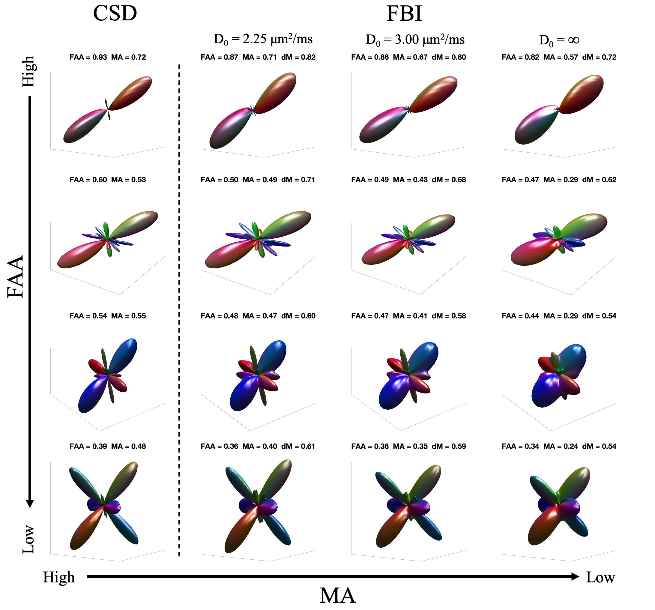
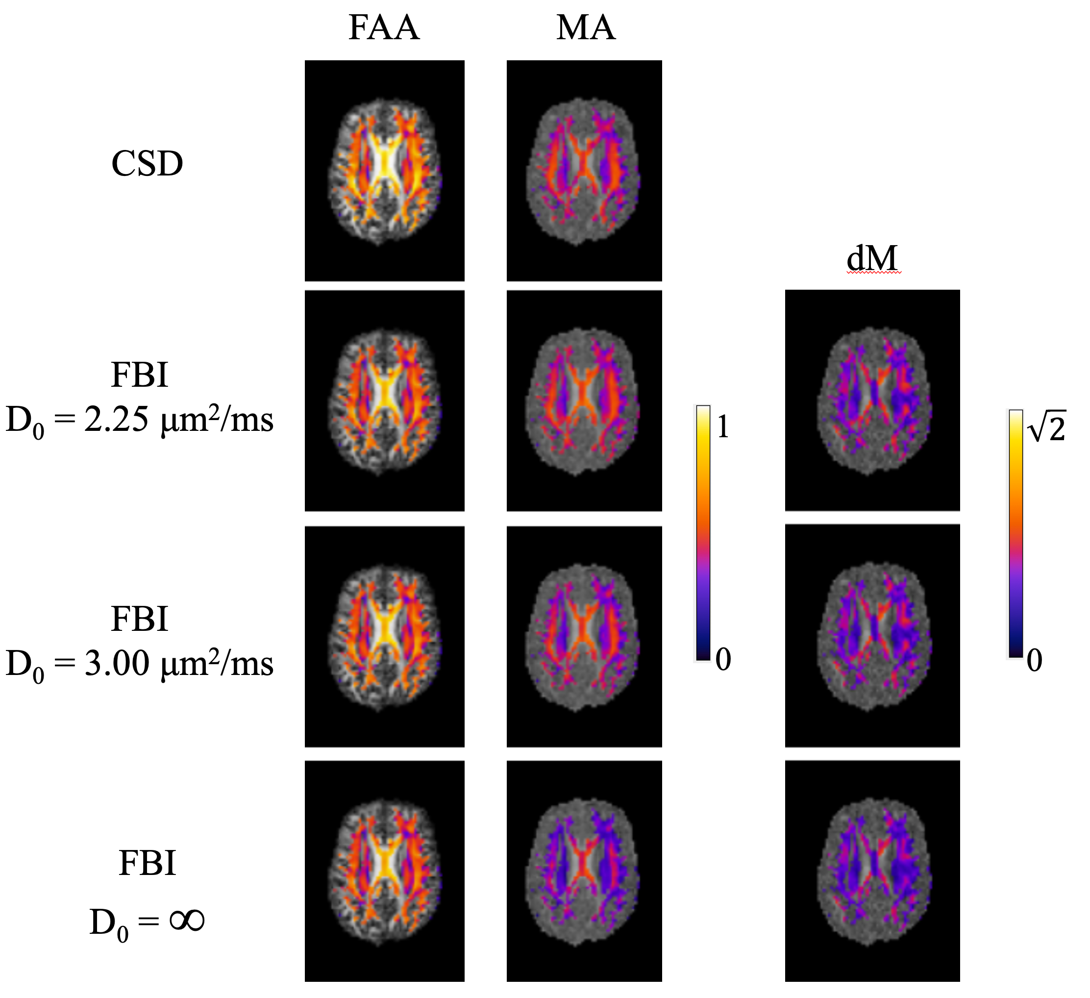
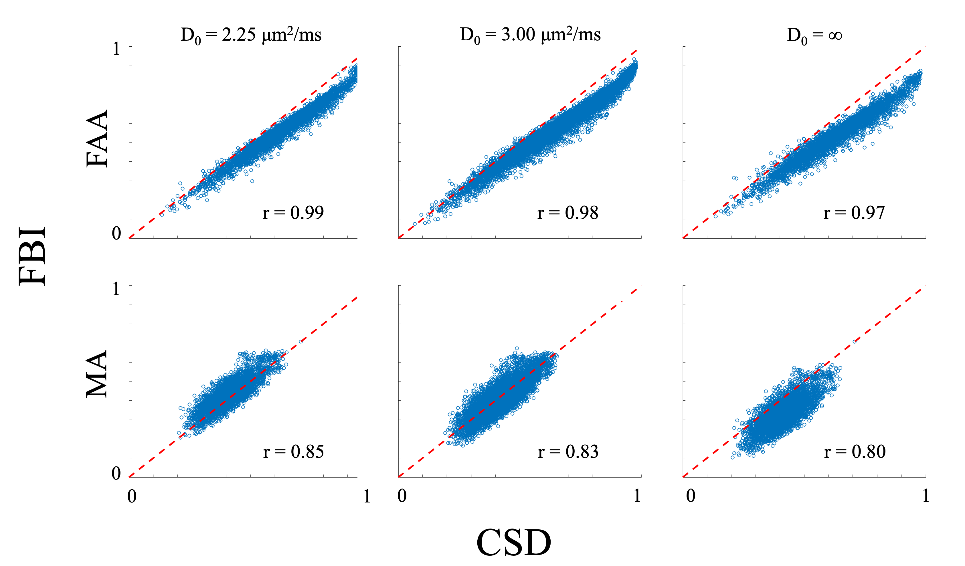
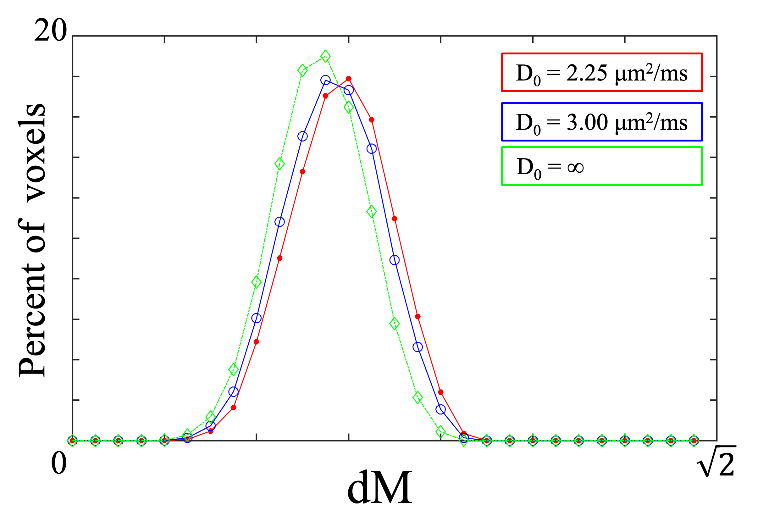
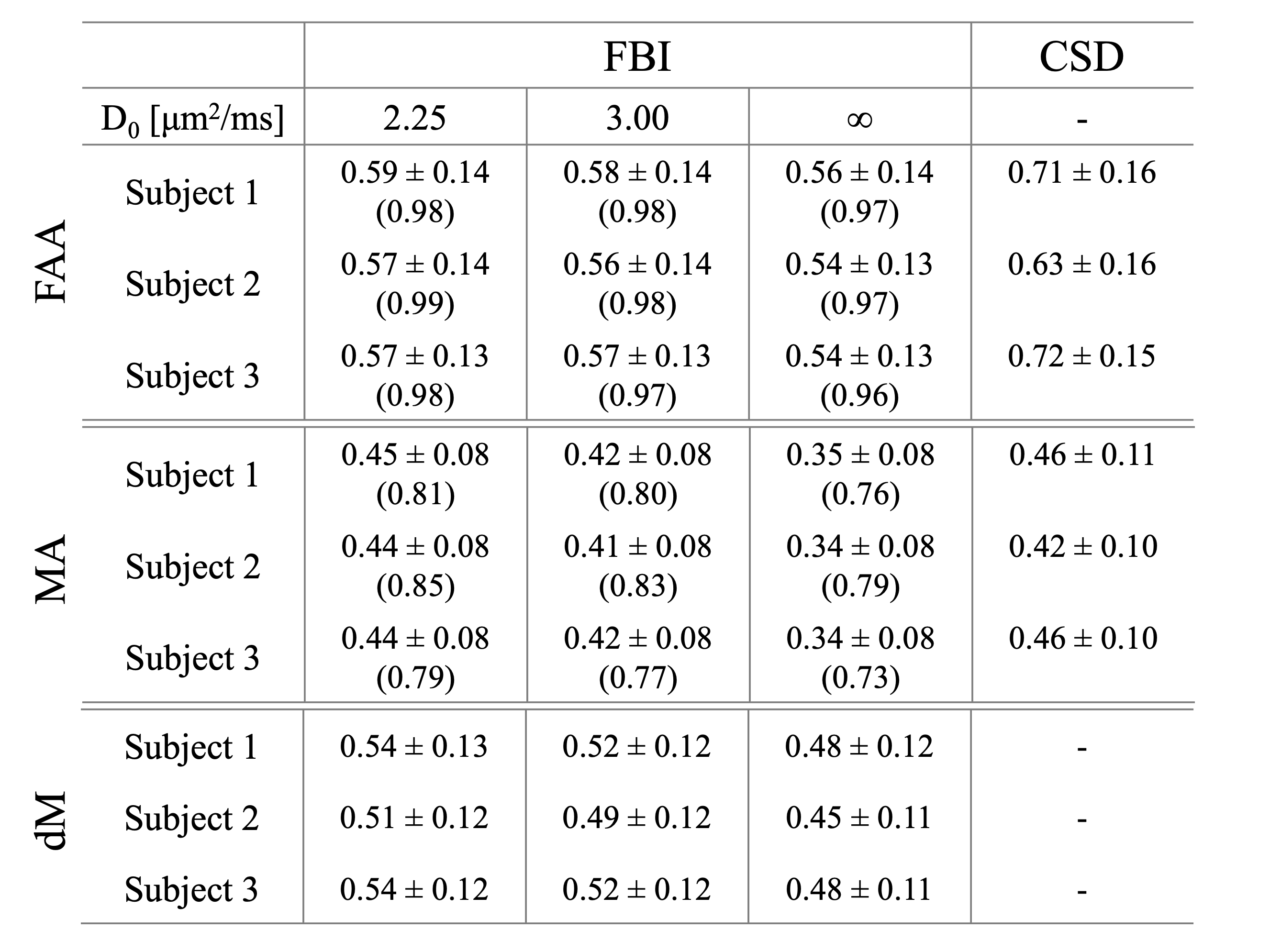
Representative fODF glyphs are presented in Figure 1 for both CSD and FBI across $$$D_{0}$$$ values, illustrating a good qualitative agreement among the fODFs. In Figure 2, FAA, MA and dM maps for an axial slice of one subject are shown where the colored regions indicate WM. For both FAA and MA, a close correspondence between CSD and FBI is apparent with $$$D_{0}$$$ = 2.25 μm²/ms but which diminishes as $$$D_{0}$$$ increases, especially for MA. In contrast, the fODF differences, dM, grow with decreasing $$$D_{0}$$$. Figure 3 gives FAA and MA scatter plots for WM voxels combined across subjects. A strong correlation between the CSD and FBI values is observed for all $$$D_{0}$$$ values, with the FAA having a higher correlation than the MA. The distribution of dM over WM voxels from all three subjects is plotted in Figure 4 for the three $$$D_{0}$$$ choices, indicating substantial differences between the CSD and FBI fODFs. Averages for FAA, MA and dM over all WM voxels for each of the three subjects are reported in Figure 5.

DISCUSSION

Despite being based on markedly different calculational schemes, fODFs obtained with CSD and FBI are strikingly similar. This is reflected by the strong FAA and MA correlations. These correlations improve with decreasing $$$D_{0}$$$ suggesting that, in terms of anisotropy, the FBI fODF for $$$D_{0}$$$ = 2.25 μm²/ms is the most similar to the CSD fODF. Nonetheless, substantial differences between CSD and FBI fODFs in most voxels are revealed by the dM, attributable to disparities in peak directions and fine structure. Interestingly, the dM increases in most voxels as $$$D_{0}$$$ is reduced, potentially from enhanced sensitivity to signal noise or sharper FBI fODF peaks that occur with a lower $$$D_{0}$$$. Sharper peaks can amplify the effect on dM of small misalignments in peak directions by reducing the extent to which CSD and FBI peaks overlap.

Acknowledgements

No acknowledgement found.

References

1. Tournier JD, Calamante F, Gadian DG, Connelly A. Direct estimation of the fiber orientation density function from diffusion-weighted MRI data using spherical deconvolution. Neuroimage. 2004;23:1176-1185.

2. Tournier JD, Calamante F, Connelly A. Robust determination of the fibre orientation distribution in diffusion MRI: non-negativity constrained super-resolved spherical deconvolution. Neuroimage. 2007;35:1459-1472.

3. Jensen JH, Glenn GR, Helpern JA. Fiber ball imaging. Neuroimage. 2016;124:824-833.

4. Moss HG, McKinnon ET, Glenn GR, Helpern JA, Jensen JH. Optimization of data acquisition and analysis for fiber ball imaging. Neuroimage. 2019;200:690-703.

5. McKinnon ET, Helpern JA, Jensen JH. Modeling white matter microstructure with fiber ball imaging. Neuroimage. 2018;176:11-21.

6. Matusita K. Decision rules, based on the distance, for problems of fit, two samples, and estimation. Ann Math Stat. 1955;26:631-640.

7. Veraart J, Novikov DS, Christiaens D, Ades-Aron B, Sijbers J, Fieremans E. Denoising of diffusion MRI using random matrix theory. Neuroimage. 2016;142:394-406.

8. Kellner E, Dhital B, Kiselev VG, Reisert M. Gibbs-ringing artifact removal based on local subvoxel-shifts. Magn Reson Med. 2016;76:1574-1581.

9. Gudbjartsson H, Patz S. The Rician distribution of noisy MRI data. Magn Reson Med. 1995;34:910-914.

10. Tournier JD, Smith R, Raffelt D, Tabbara R, Dhollander T, Pietsch M, Christiaens D, Jeurissen B, Yeh CH, Connelly A. MRtrix3: A fast, flexible and open software framework for medical image processing and visualisation. Neuroimage. 2019;202:116137.

11. Dhital B, Reisert M, Kellner E, Kiselev VG. Intra-axonal diffusivity in brain white matter. Neuroimage. 2019;189:543-550.

12. Moss HG, Jensen JH. Optimized rectification of fiber orientation density function. Magn Reson Med. 2021;85:444-455.

Figures

Representative fODF glyphs from CSD and FBI for $$$D_{0}$$$ = 2.25, 3.00 and $$$\infty$$$ μm²/ms and with each row corresponding to a unique WM voxel. Rows are ordered from high (top) to low (bottom) FAA values while columns are ordered from high (left) to low (right) MA values. The FAA and MA differ in that the FAA is only sensitive to spherical harmonics of degree 2 and lower, while the MA depends on all spherical harmonics. Notice that there is good qualitative accord among all fODFs for a given voxel. The quantitative differences are further explored in this study.

Parametric maps, for a single axial slice, of the FAA, MA and dM that compare fODFs estimated by CSD and FBI at three different diffusivity reference values, $$$D_{0}$$$ = 2.25, 3.00 and $$$\infty$$$ μm²/ms. The colored regions indicate WM voxels used in the calculations. The FAA maps for CSD and FBI are similar for all values of $$$D_{0}$$$. The CSD and FBI MA maps are also similar with $$$D_{0}$$$ = 2.25 μm²/ms, but differences can be seen for larger $$$D_{0}$$$ values. The dM increases as $$$D_{0}$$$ is reduced and shows a strong regional variability.

The FAA and MA, as obtained with FBI, versus the CSD predictions for all WM voxels combined from three subjects. Strong correlations (r) are observed for both anisotropies, with FAA having a higher correlation than MA. The strongest correlation, for each type of anisotropy, occurs with $$$D_{0}$$$ = 2.25 μm²/ms. The dashed red line has a slope of one and indicates perfect agreement between FBI and CSD.

Distribution of dM values for all WM voxels from three subjects. The y-axis is the percent of voxels when using a bin size of 0.05. Substantial differences are apparent for all three values of $$$D_{0}$$$ with the average difference being smallest for $$$D_{0}$$$ = $$$\infty$$$ (green curve). These dM differences reflect discrepancies the peak directions and fine structure of the CSD and FBI fODFs.

Mean value ± standard deviation for each subject’s FAA, MA, and dM values. Correlation coefficients between FBI and CSD are indicated inside the parentheses for FAA and MA. The CSD FAA is somewhat larger than the FBI FAA. The CSD and FBI have comparable MA values for $$$D_{0}$$$ = 2.25 μm²/ms, but the FBI MA is somewhat lower for $$$D_{0}$$$ = 3.00 and $$$\infty$$$ μm²/ms. The mean dM values are approximately 0.50 which is roughly 35% of the maximum possible difference of $$$\sqrt{2}$$$.

Proc. Intl. Soc. Mag. Reson. Med. 29 (2021)

4286