Introduction

Ultrashort echo time (UTE) sequences have been used for cortical bone water imaging and quantification in order to acquire useful magnetic resonance (MR) signals¹. The T₁ is a useful biomarker for the cortical bone porosity and age related deterioration assessment and is also a sensitive biomarker for monitoring temperature change in cortical bone^2,3. Recently, we proposed a 3D UTE based actual flip angle imaging (AFI)-variable TR (VTR) (UTE-AFI-VTR) method for accurate cortical bone T₁ measurement⁴. The UTE-AFI-VTR method can achieve accurate measurement of the T₁ of cortical bone without degradation from the inefficient RF excitation of clinical scanners⁴. However, the scan time of the UTE-AFI-VTR sequence was relatively long for clinical practice because the UTE-VTR dataset with multiple TRs were required. To improve the time efficiency for accurate cortical bone T₁ measurement, we proposed a generalized optimization framework which simultaneously fits the UTE-AFI and the UTE with a single TR (UTE-STR) data sets to estimate T₁. This method would significantly reduce the total scan time for T₁ measurement.

Methods

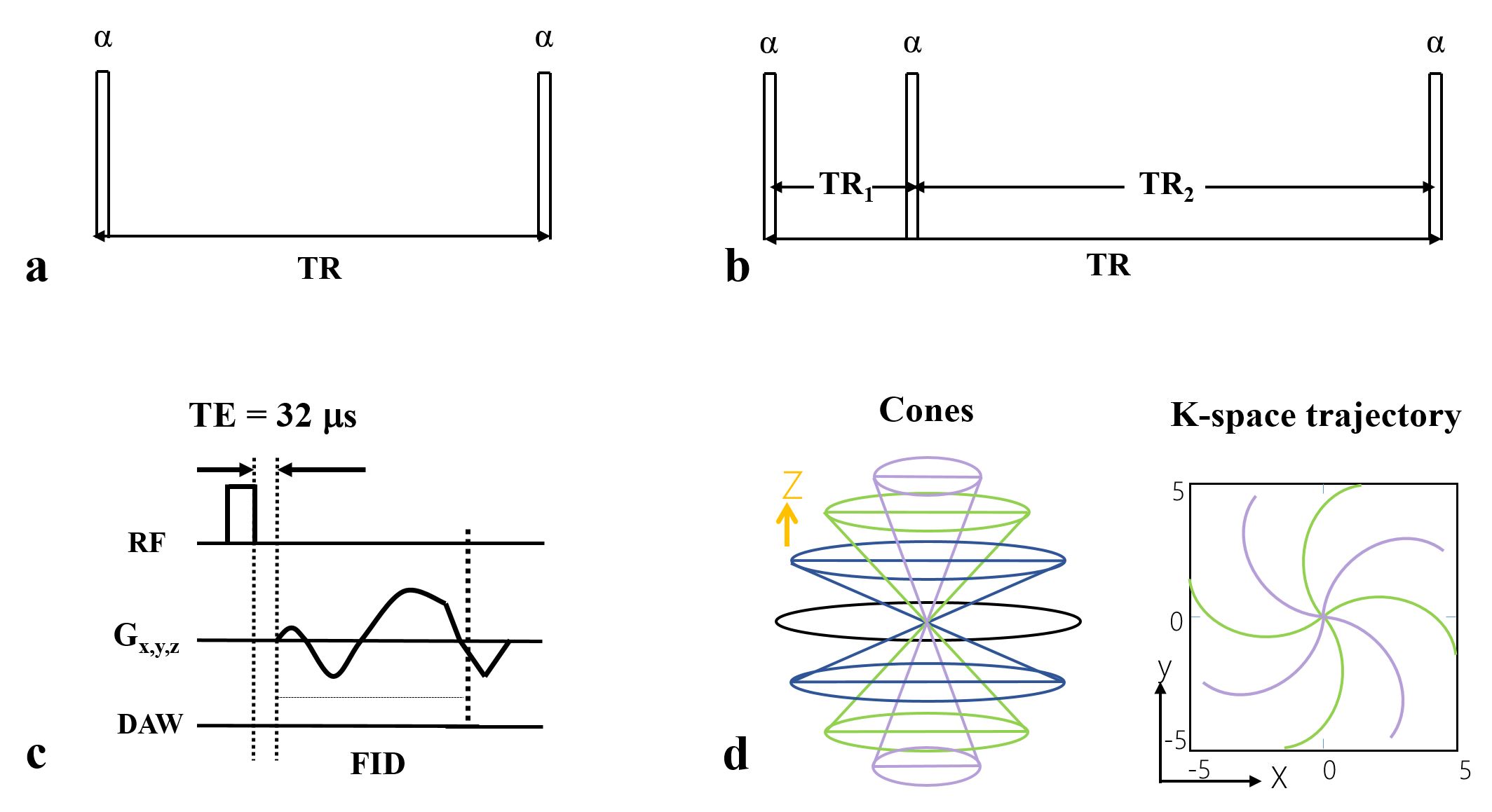
The features of the 3D UTE-AFI and UTE-VTR sequences are shown in Figure 1⁴. A short rectangular RF pulse (duration 150 μs) is used for signal excitation and this is followed by a spiral trajectory data acquisition with 3D conical view ordering in these two sequences. For ultrashort T₂ tissue excitation, the steady-state signals in TR₁ and TR₂ of the 3D UTE-AFI sequence conform to the signal models described by Eqs. [1] and [2] in reference 4. The signal detected by the 3D UTE sequence is described by Eq. [9] in reference 4. In addition, since the equilibrium magnetization M₀ and transverse magnetization mapping function generated by the RF pulse F_xy are independent of TR, they can be combined into a single unknown parameter (e.g., κ). As a result, when the RF pulse and flip angle (FA) used in the AFI and VTR sequences are identical, there are only three unknown parameters (i.e., κ, T₁, F_z) in these signal models to fit. Therefore, we can use the optimization framework below to simultaneously fit (sf) UTE-AFI and UTE-VTR (sf-UTE-AFI-VTR) data:
$$\left[\kappa~T_{1}~F_{z}\right]=\text{arg}\min\limits_{\kappa,T_{1},F_{z}}\left\{\sum_{i=1}^2[I_{AFI,i}-S_{AFI,i}]^2+\sum_{j=1}^N[I_{VTR,j}-S_{VTR,j}]^2\right\}~~~~~~~[1]$$
where $$$\text{arg}\min\limits_{x}\left(y(x)\right)$$$ means finding a $$$x$$$ value which can make $$$y(x)$$$ attain its minimum value. $$$I_{AFI,i}$$$ ($$$i$$$ = 1 and 2) and $$$I_{VTR,j}$$$ ($$$j$$$ = 1,2,..., N) are the sampled signal intensities from the UTE-AFI and UTE-VTR sequences respectively. $$$S_{AFI,i}$$$ and $$$S_{VTR,j}$$$ are the signal models of the UTE-AFI and UTE-VTR sequences respectively⁴. N is the total number of TRs. $$$\kappa=M_{0}F_{xy}\left(\alpha,\tau,T_{2}\right)$$$. This framework simultaneously yields a solution for the three unknown parameters: κ, T₁, and F_z. Since there are only three unknown parameters in Eq. [1], a single regular UTE acquisition together with the other two UTE-AFI acquisitions is sufficient to estimate them using the optimization framework. To save scan time, we therefore propose a UTE-AFI-STR method (i.e., a combination of the UTE-AFI and UTE-STR methods) to provide accurate measurement of T₁.
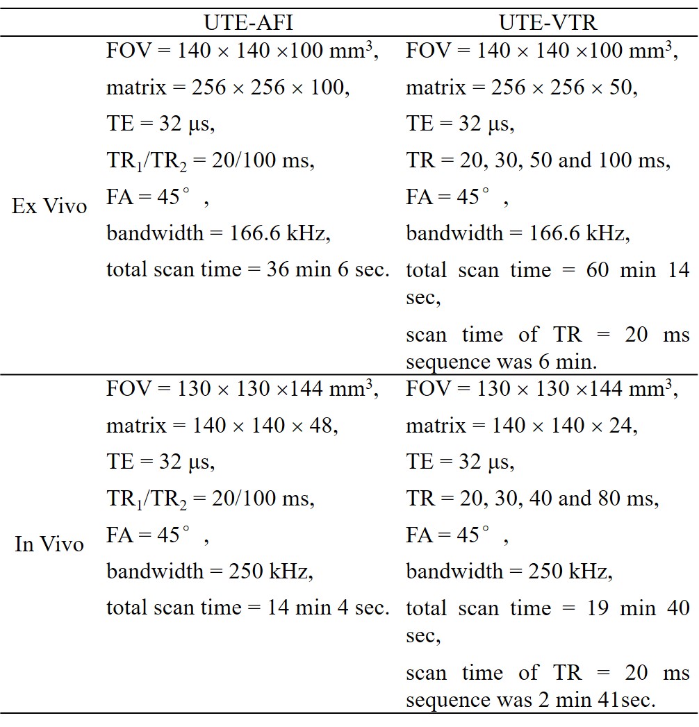
Numerical simulations, ex vivo and in vivo human cortical bone experiments were conducted to demonstrate the accuracy of the proposed fast 3D UTE-AFI-STR method. In simulations, T₁ maps generated with the UTE-AFI-VTR, sf-UTE-AFI-VTR, and UTE-AFI-STR methods were compared at different SNR levels and the error ratios were calculated. The UTE-AFI and UTE-VTR sequences were performed on nine human cortical bone samples (aged from 38 to 95 years, 5 females) and four healthy volunteers (35±16 years, 3 males) and their T₁ maps were calculated with the aforementioned three methods. The T₁ value difference errors between the UTE-AFI-STR and the UTE-AFI-VTR/sf-UTE-AFI-VTR methods were calculated as well. The parameters used in the simulations were the same as in vivo experiments and the sequence parameters of ex vivo and in vivo experiments are shown in Table 1. The total scan times of the UTE-AFI-STR method were about 54 minutes and 17 minutes less than the UTE-AFI-VTR/sf-UTE-AFI-VTR methods in the ex vivo and in vivo experiments, respectively.

Results and Discussion

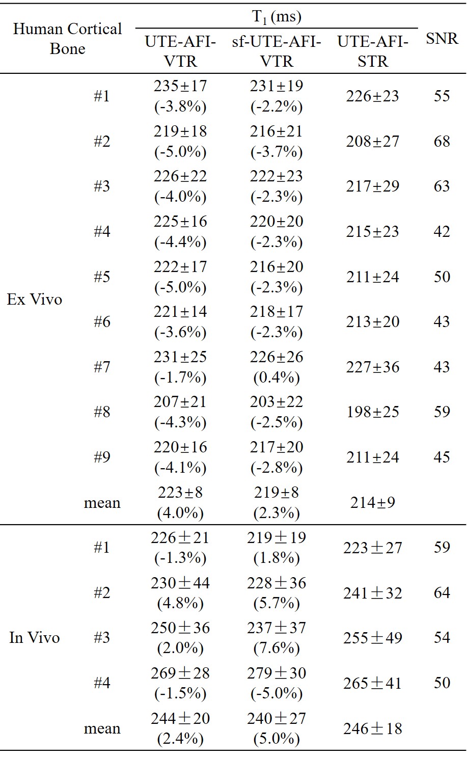
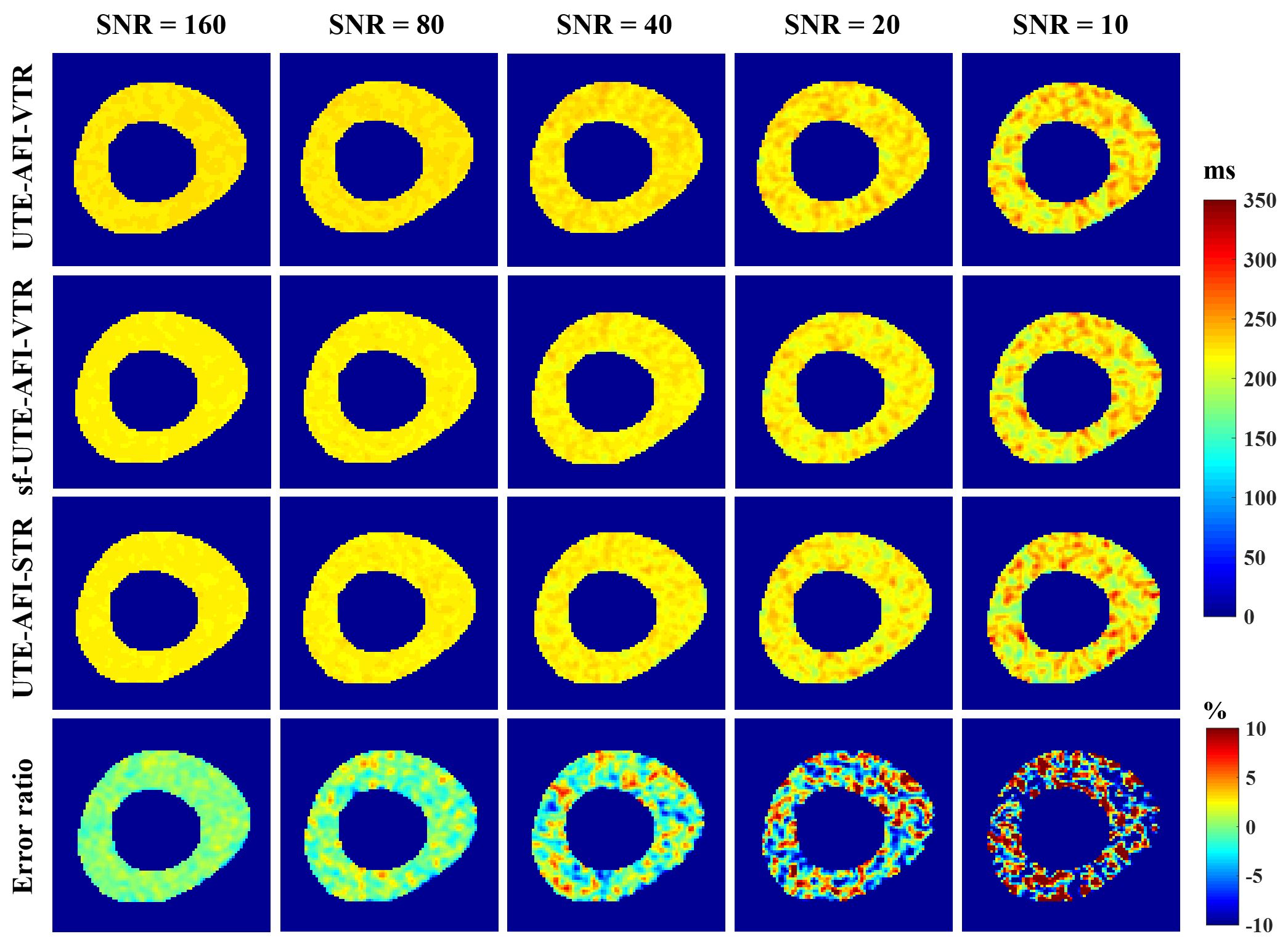
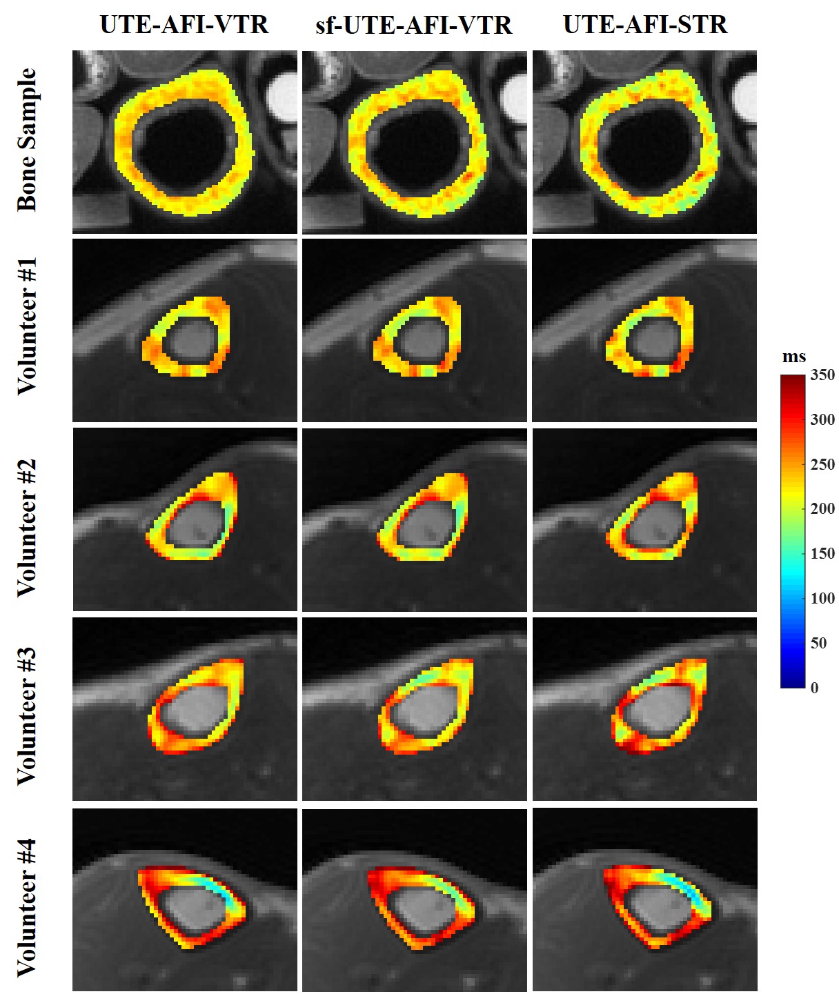
As shown in Figure 2, when the signal to noise ratio (SNR) of UTE-STR image was higher than 40, the T₁ value derived from UTE-AFI-STR method was close to the standard T₁ (i.e., 220 ms) (error ratios ranged from -5% to 5%). This observation shows that the fast UTE-AFI-STR method is accurate for T₁ measurement when the SNR of the UTE-STR image is higher than 40.
In Figure 3, the T₁ maps of ex vivo and in vivo cortical bones obtained with three methods looked similar. In Table 2, the T₁ value difference ratios between range between -5.0% and 0.4%, and -5.0% to 7.6% for ex vivo and in vivo measurements, respectively. The average cortical bone T₁ for the four volunteers calculated using the UTE-AFI-STR method was 246 ms, which is similar to previously reported values^5-7. These observations demonstrate the accuracy and good agreement of the T₁ measurement of the UTE-AFI-STR method as compared with the other two methods which require much more scan time.

Conclusion

The proposed 3D UTE-AFI-STR method provides accurate T₁ mapping of cortical bone with improved time efficiency compared with the UTE-AFI-VTR/sf-UTE-AFI-VTR methods.

Acknowledgements

The authors acknowledge grant support from GE Healthcare, NIH (R01AR068987, R01NS092650, and R21AR075851) and scholarship support from the Joint Ph.D. Training Program of the University of Chinese Academy of Sciences (UCAS).