Introduction

The concept of balanced steady-state free precession (bSSFP) has been first introduced by Carr¹ in the late 1950s in the context of spectroscopy. Since then it has become increasingly popular for imaging due to its high signal efficiency and its $$$T_2/T_1$$$-weighted contrast.
Although its signal properties have been extensively investigated, it was only noted about a decade ago by Miller² that for bSSFP various tissues exhibit a strong and rather unexpected asymmetry in the frequency profile. Generally, the observed asymmetry in tissues arises from local intra-voxel frequency distributions driven by its rich and complex underlying microstructure. This effect is especially strong in brain tissue where myelination leads to a frequency dispersion. In this work, we use configuration theory to show that, generally, tissues forget about their spectral composition when using bSSFP imaging in the limit of $$$\mathit{TR}\rightarrow 0$$$. It is shown that this holds true for $$$\mathit{TR}\sim1\,\mathrm{ms}$$$ at $$$3\,\mathrm{T}$$$.

Theory

We consider the spin density $$$M$$$ being composed of a normalized spectrum of magnetizations $$$m_k$$$ with associated chemical shifts $$$\delta_k$$$. We now look at a train of RF pulses with equidistant spacing given by $$$\mathit{TR}$$$ and linear RF phase increase $$$\varphi_j=-j\phi$$$ for the $$$j$$$th $$$\mathit{TR}$$$ interval, where $$$\phi$$$ is the phase increase per $$$\mathit{TR}$$$. The magnetization immediately after the RF pulse can be expressed as a series over all configuration orders and spectral components:
$$M(\phi,k)=\sum_{n,k} e^{in(\theta_k + \phi)}m_k^{(n)}\tag{1}$$
where $$$\theta_k=2\pi\gamma B_0\delta_k\mathit{TR}$$$ denotes the phase accumulation of $$$m_k$$$ within any $$$\mathit{TR}$$$ at some given main magnetic field strength $$$B_0$$$.
We immediately see that $$$\lim\limits_{\mathit{TR}\rightarrow 0}\theta_k=0$$$ and therefore
$$\lim\limits_{\mathit{TR}\rightarrow 0}M(\phi,k)=\sum_{n,k}e^{in\phi}m_k^{(n)}=\sum_{n=-\infty}^{\infty}e^{in\phi}\left(\sum_{k=0}^{K}m_k^{(n)}\right)=\sum_{n=-\infty}^{\infty}e^{in\phi}M^{(n)}=M(\phi).\tag{2}$$
This means the voxel eventually ''forgets'' about its spectral composition, having the apparent properties of a ''pure'' voxel. For the $$$2\pi$$$ periodicity of the bSSFP frequency response function the ''purity'' condition
$$2\pi\gamma B_0\delta_k\mathit{TR}\approx0\tag{3}$$
implies
$$\delta_k\ll\frac{1}{\gamma B_0\mathit{TR}}\hspace{.5cm}\mbox{or}\hspace{.5cm}\mathit{TR}\ll\frac{1}{\gamma B_0\delta_k}\label{limits}\tag{4}$$
Notably this becomes less stringent with decreasing $$$B_0$$$ for fixed $$$\delta_k$$$.
For brain tissue a frequency dispersion of about $$$20\,\mathrm{Hz}$$$ was observed at $$$3\,\mathrm{T}$$$ ², leading to a limit of $$$\mathit{TR}\ll50\,\mathrm{ms}$$$. On modern scanners a $$$\mathit{TR}$$$ of $$$1-2\,\mathrm{ms}$$$, which is expected to fulfill the limit, can generally be reached for reasonable resolutions, therefore opening the possibility to validate the theory.

Methods

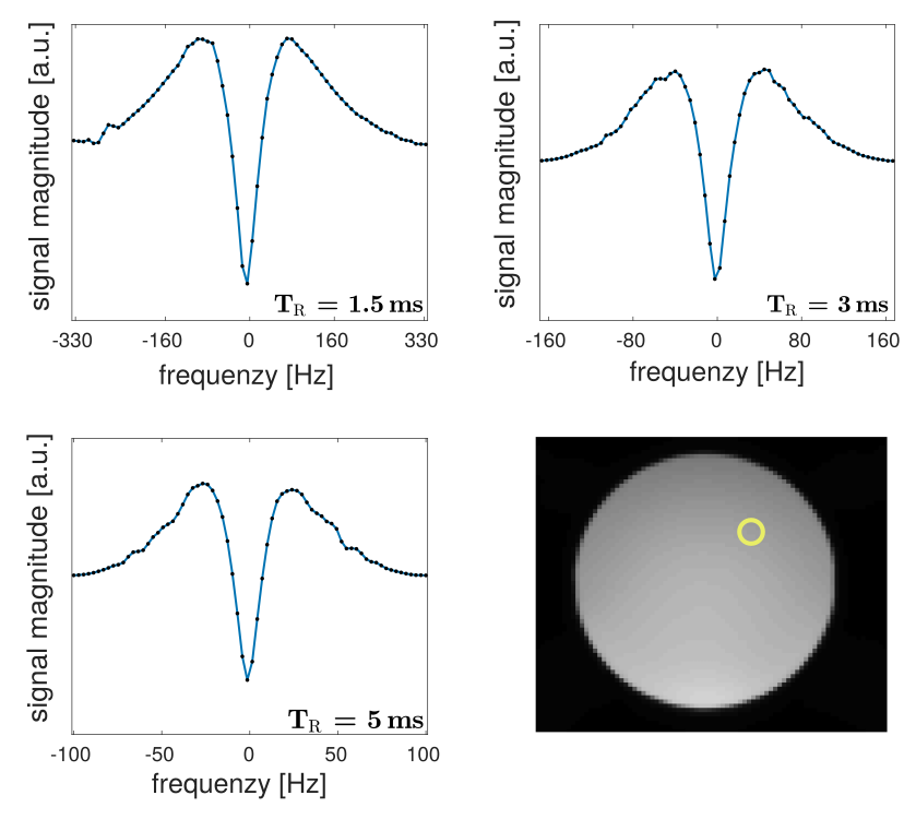
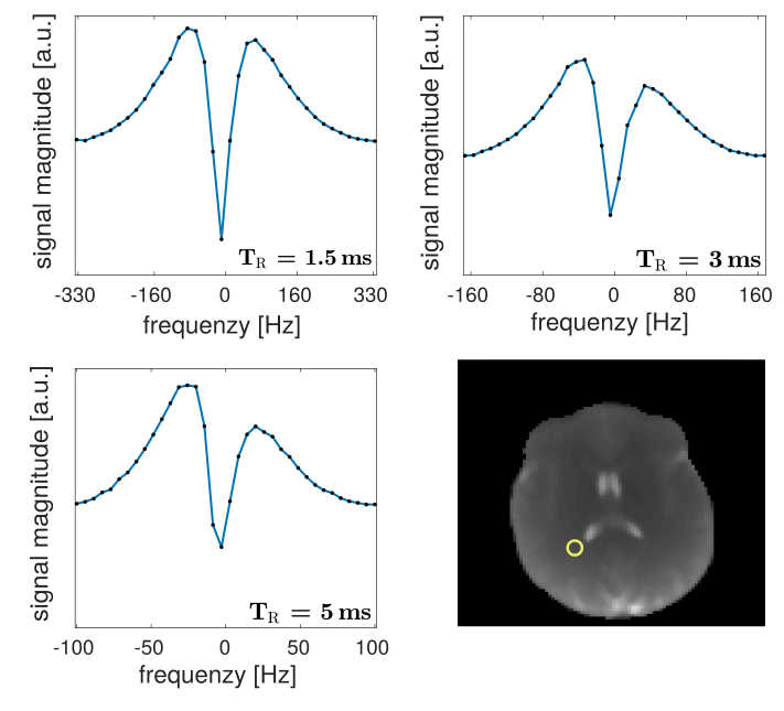
Imaging was performed at $$$3\,\mathrm{T}$$$ using a slightly modified standard cartesian bSSFP sequence with automated phase-cycling and optional reversed sweep direction. Scans were performed for pure spin densities using a manganese-doped, aqueous phantom $$$(T_1=860\,\mathrm{ms},T_2=70\,\mathrm{ms})$$$ and for in vivo brain where a strong profile asymmetry is expected³.
Non-selective bSSFP imaging was performed with a nominal flip angle of $$$\alpha=10^{\circ}$$$ for three different values of $$$\mathit{TR}\,(1.5\,\mathrm{ms},3.0\,\mathrm{ms},5.0\,\mathrm{ms})$$$ with corresponding bandwidths of $$$\{1775,610,270\}\,\mathrm{Hz/Px}$$$. A field-of-view of $$$256$$$ with $$$75\%$$$ resolution in phase direction, a base resolution of $$$128$$$ and a slice thickness of $$$2.0\,\mathrm{mm}$$$ were chosen, resulting in an imaging matrix of $$$128\times96\times80$$$ and an isotropic resolution of $$$2.0\,\mathrm{mm}$$$. For each $$$\mathit{TR}$$$ setting, $$$N$$$ scans with equally distributed linear RF phase increments in the interval $$$[0,2\pi)$$$ were recorded. A dummy preparation period of $$$3-5\,\mathrm{s}$$$ was used to ensure steady-state conditions. The phantom scans were performed with $$$N = 72$$$, the brain scans with $$$N = 36$$$.
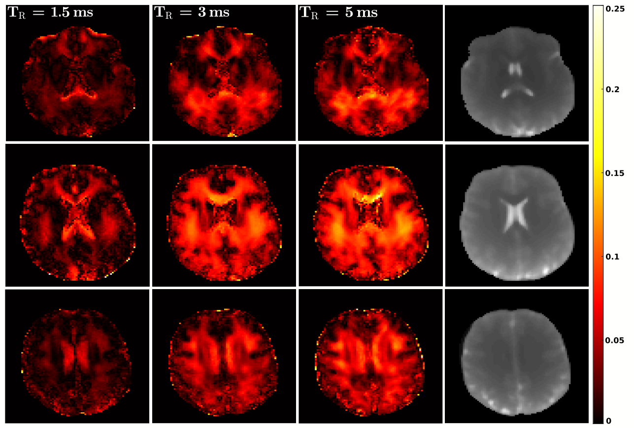
Scanning took $$$20\,\mathrm{min}$$$ $$$(\mathit{TR}=1.5\,\mathrm{ms}$$$ and $$$\mathit{TR}=3\,\mathrm{ms})$$$ and $$$24\,\mathrm{min}$$$ $$$(\mathit{TR}=5\,\mathrm{ms})$$$, respectively, for the phantom and $$$10\,\mathrm{min}$$$ $$$(\mathit{TR}=1.5\,\mathrm{ms}$$$ and $$$\mathit{TR}=3\,\mathrm{ms})$$$ and $$$12\,\mathrm{min}$$$ $$$(\mathit{TR}=5\,\mathrm{ms})$$$, respectively, for the brain scan to complete. For the brain scans the asymmetry index $$$(\mathit{AI})$$$ was calculated as stated in Miller et. al.³ via
$$\mathit{AI} = \frac{h_p-h_n}{h_p + h_n}\tag{5}$$
where $$$h_{p,n}$$$ is the peak signal at the positive ($$$p$$$) or negative ($$$n$$$) frequency offset from the center.

Results & Discussion

For the phantom scans (Fig. 1), the observed frequency response of bSSFP is symmetric for all $$$\mathit{TR}$$$, as can be expected for pure voxels with symmetric frequency dispersions. This is in contrast to the findings for brain white matter (Fig. 2). Here, a pronounced asymmetry is observed for a $$$\mathit{TR}$$$ of $$$5\,\mathrm{ms}$$$, in agreement with previous findings². The asymmetry index, however, becomes markedly attenuated with a decrease in $$$\mathit{TR}$$$, as is evident from the figure. $$$\mathit{AI}$$$ maps are shown in Fig. 3 for three axial slices. A morphological image is shown as reference. As reported by Miller et. al.³ a rich variation of the $$$\mathit{AI}$$$ is observed for brain tissue, with highest $$$\mathit{AI}$$$ values in the corpus callosum, while the region around the corticospinal tract exhibits generally the lowest asymmetry. Overall, the $$$\mathit{AI}$$$ maps show a pronounced sensitivity on the $$$\mathit{TR}$$$ and decrease with decreasing $$$\mathit{TR}$$$, as expected from theory (please note that the cerebrospinal fluid would require at least three times $$$T_1$$$ to yield a symmetric response and thus the observed residual asymmetry reflects transient effects). Consequently, for a $$$\mathit{TR}$$$ of about $$$1\,\mathrm{ms}$$$, bSSFP imaging of brain tissue becomes apparently pure at $$$3\,\mathrm{T}$$$. This limit will become less stringent at lower fields (cf. Eq.4) and pure bSSFP imaging of tissues will become feasible with clinically relevant resolutions, e.g. at $$$1.5\,\mathrm{T}$$$ using a $$$\mathit{TR}\sim2\,\mathrm{ms}$$$.

Conclusion

We have shown that the pronounced asymmetry in the bSSFP frequency response profile, stemming from intra-voxel frequency distributions, vanishes for $$$\mathit{TR}\rightarrow0$$$. At $$$3\,\mathrm{T}$$$, the asymmetry vanishes for $$$\mathit{TR}\sim1\,\mathrm{ms}$$$, whereas at lower clinical field strength, such as $$$1.5\,\mathrm{T}$$$, pure bSSFP imaging is expected for $$$\mathit{TR}\sim2\,\mathrm{ms}$$$ and thus becomes feasible for clinically relevant resolutions.

Acknowledgements

This work was supported by the Swiss National Science Foundation (SNF grant No. 325230_182008).