4184
A Revised Algorithm for Spiral Gradient Waveforms with a Compact Frequency Spectrum
James Pipe1
1Mayo Clinic, Rochester, MN, United States
1Mayo Clinic, Rochester, MN, United States
Synopsis
This work presents a versatile new algorithm to design better spiral trajectories, by minimizing high spatial frequencies in the gradient waveform and dynamically compensating for preconditioning by adaptively changing the maximum gradient and slew rate limits. It has been integrated into software, and example waveforms are given.
Introduction
Spiral MRI has high SNR AND temporal efficiency, incoherent aliasing and motion artifacts, flexibility for sequence design, and low minimum TE. Despite these benefits, spiral trajectories are not widely used clinically, notably because they generally lack robustness to both B0 inhomogeneities as well as gradient (trajectory) imperfections. This work addresses gradient waveform design given the limits of a gradient system transfer function, which tends to dampen higher spatial frequencies (acts as a low-pass filter). This creates trajectory errors which, if not corrected for, resulting in mis-mapping of collected data and subsequent image artifacts.Typically this high-frequency dampening behavior is addressed by some combination of (a) measuring or predicting the actual trajectory and (b) precompensating the waveform by enhancing the higher frequencies by the inverse of the transfer function. Trajectory measurement alone is not an ideal solution when one prefers to collect data on the designed trajectory. Precompensated waveforms often exhibit gradient amplitude or slew spikes which, when scaling the precompensated waveform to match system performance, result in an "underperforming" waveform.
This work illustrates a new method to place a frequency limit on a designed spiral waveform, and also introduces the concept of frequency preconditioning, so that the precompensated waveform is optimally matched to the system limits.
Theory
FREQUENCY LIMITINGLimitations on the instantaneous frequency of spiral waveforms have previously been described (1). This work builds on the numerical Spiral algorithm presented in (2), which is different than that in (1). Math shows that instantaneous frequency limits can be imposed by limiting the gradient amplitude |g| by
$$g_m= f_{cap}\frac{RN}{\gamma F} \frac { (\tilde{\phi} ^2 + 1) ^{3/2}}{\tilde{\phi} ^2+2}$$
and slew amplitude |s| by
$$s_m= 2\pi f_{cap} g_m \sqrt{1+\frac { \tilde{\phi}^2(\tilde{\phi} ^2 + 4) ^2}{(\tilde{\phi} ^2+2)^4} },$$
where fcap, R, N, $$$\gamma$$$, and F are the maximum desired frequency, undersampling ratio, # arms for a fully sampled spiral, gyromagnetic ratio, and FOV, and
$$\tilde{\phi}(k_r)=\frac{2\pi F}{R(k_r)N} k_r,$$
where kr is the kspace radius.
TRANSITION SMOOTHING
As in (1), the spiral waveform is divided into frequency-limited, slew-limited, and gradient-limited regimes, each with their own set of gradient and slew limits. The transitions between each regime are calculated, and the gradient and slew limits (before and after transition) are blended to smooth the discontinuities in the gradient waveform, further minimizing the high frequencies in the waveform.
PRECOMPENSATION CONDITIONING
In a smooth waveform, the instantaneous gradient frequencies represent the great majority of the waveform's frequency content. During the numerical design of the waveform, gradient and slew limits are dynamically reduced by 1/GTF(fI), where GTF is the gradient transfer function and fI is the calculated instantaneous frequency of the gradient waveform. With a smooth waveform, the precompensation that occurs after waveform design with this conditioning will produce a waveform that (nearly) exactly matches system gradient amplitude and slew limits.
Methods
SOFTWAREThe software in (2) was modified to implement the frequency limiting, transition smoothing, and precompensation conditioning mentioned above. Additional waveform smoothing was added by using a temporal Hanning window on gradient limits at the beginning of the waveform, and a Hanning window design for gradient rampdown after the end of the spiral trajectory. The gradient impulse response function (GIRF) for a particular gradient set is input numerically, and the resulting GTF is calculated by FFT. Waveform precompensation is performed in the code via numerical deconvolution. Spiral-in waveforms are computed as spiral-out waveforms, then flipped in time prior to precompensation.
EXAMPLE WAVEFORMS
To illustrate the performance of the algorithm, several waveforms were generated, using the parameters given in Fig. 1. The Standard spiral (see Fig. 1) was generated with different layers of the proposed technology, adding frequency limiting, then transition smoothing, and then precompensation conditioning, to the initial design. The other waveforms were only generated using all of the proposed technology. For each case, both the designed and precompensated gradient waveforms were generated, along with the k-space trajectory. A synthesized GIRF given by a Gaussian curve, illustrated in Fig. 2(a), with its GTF in Fig. 2(b), was used for precompensation and conditioning.
Results
K-space trajectories for each waveform are shown in Fig 2(c-f). The designed and precompensated waveforms for the Standard spiral are shown in Fig 3, showing how each layer of the proposed method reduces the spikes in slew rate in the precompensated waveform, until (Fig. 3d) the precompensated waveform is within system limits. The other waveforms are shown in Fig 4, illustrating the versatility of the method. The single shot method does show a spike above system limits at the end of the waveform.Conclusion
The proposed method introduces two new technologies. First, it presents a versatile new algorithm to limit the gradient frequency which fits well with numerous spiral waveform algorithms, including that used in this work. Second, it introduces the concept of dynamic precompensation conditioning, which maximizes the performance (reduces overall time) by keeping the precompensated waveform as close to the maximum system limits as possible. The spike seen in the precompensated waveform of Fig 4(c) is likely due to the transition from the "maximum slew" regime to the gradient rampdown, skipping the "maximum gradient amplitude" regime, and represents an area for improvement in the software/algorithm design.Acknowledgements
This work was funded in part by Philips Healthcare.References
1. Oberhammer T, Weiger M, Hennel F. Spiral MRI trajectory design with frequency constraint. Proceedings of the Joint Annual Meeting of ISMRM-ESMRMB 2010;p. 4969.
2. Pipe JG, Zwart NR. Spiral Trajectory Design: A Flexible Numerical Algorithm and Base Analytical Equations. Magn Reson Med 2014;71(1):278–85.
Figures
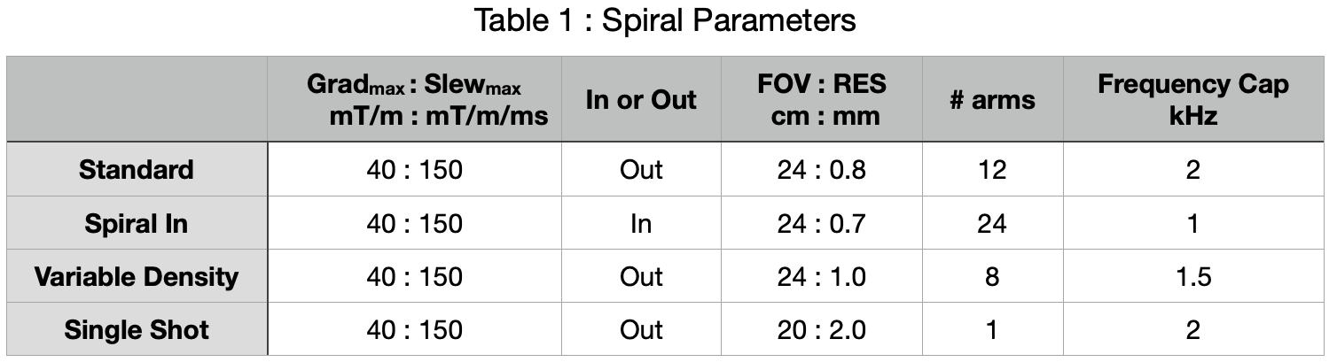
Parameters of the four waveforms designed and illustrated in this work. For the variable density spiral, the arm spacing was defined to be critical (R=1) for kr < 20% maximum, and transitioned with a Hanning window to an undersampling factor of R=3 at normalized kr = 50% maximum and above.
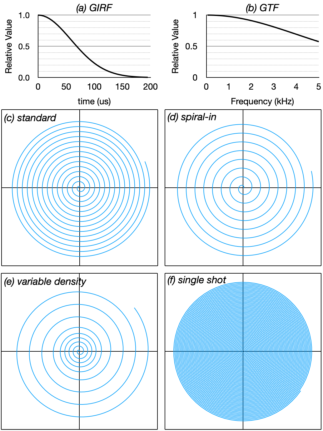
Illustration of the (a) GIRF and (b) GTF used for precompensation and conditioning used in this work, and (c-f) the k-space trajectories for a single arm from each of the four waveforms specified in Figure 1.
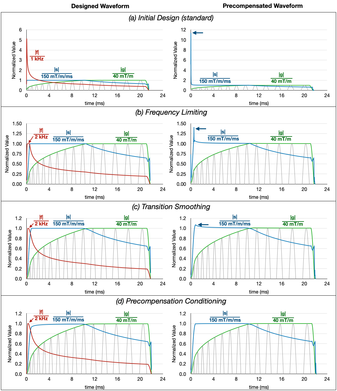
Designed (left) and precompensated (right) waveforms for the Standard trajectory, from (a) the initial design, then adding (b) frequency limiting, (c) transition smoothing, and (d) precompensation conditioning. Frequency, slew, and gradient amplitude waveforms are colored red, blue, and green, while the gray waveforms show the positive part of Gx. The blue arrows illustrate the spikes in the slew rate of the precompensated waveforms, which are further mitigated with each layer. Waveforms are normalized by the design maximum for easier visualization.
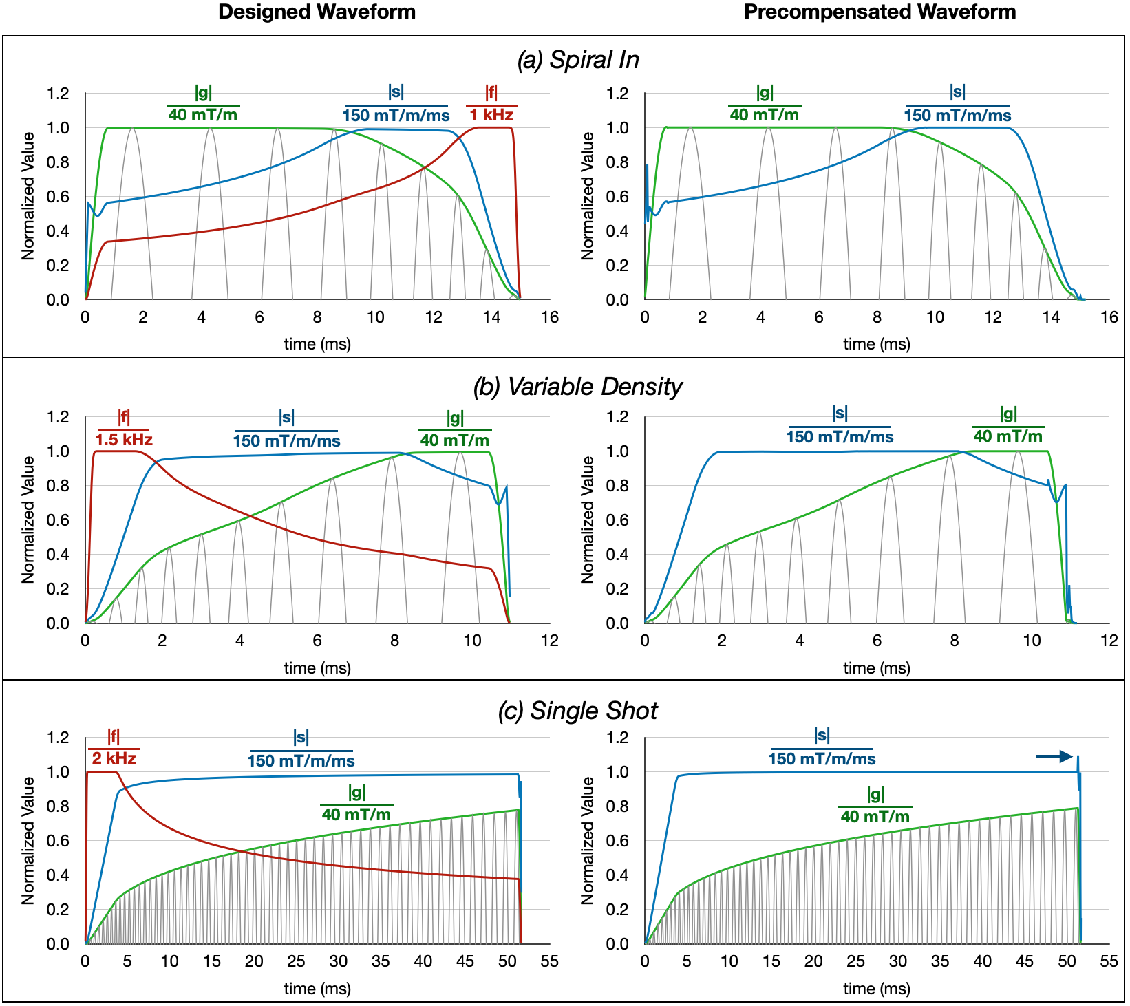
Designed (left) and precompensated (right) waveforms for the (a) spiral-in, (b) variable density, and (c) single shot trajectories. Frequency, slew, and gradient amplitude waveforms are colored red, blue, and green, while the gray waveforms show the positive part of Gx. Waveforms are normalized by the design maximum for easier visualization.