4165
High-resolution, low-SAR 3D T2 relaxometry with COMBINE1Department of Brain Sciences, Imperial College London, London, United Kingdom, 2Department of Surgery and Cancer, Imperial College London, London, United Kingdom, 3Department of Imaging, Imperial College Healthcare NHS Trust, London, United Kingdom, 4Department of Bioengineering, Imperial College London, London, United Kingdom, 5MRC London Institute of Medical Sciences, London, United Kingdom, 6UK Dementia Research Institute Centre at Imperial College, London, United Kingdom, 7Wellcome Centre for Integrative Neuroimaging, Nuffield Department of Clinical Neurosciences, University of Oxford, Oxford, United Kingdom
Synopsis
Here we describe a super-resolution 3D T2 relaxometry approach using an unbalanced SSFP acquisition with very low flip angle RF pulses (α ≤ 1°). We then apply this to obtain 1mm isotropic T2 maps in a reference phantom, and compare this to both the reference values and a 2D multi-echo spin echo approach. The proposed approach provides new options for high-resolution, low-SAR T2 relaxometry experiments in a range of tissues.
Introduction
High-resolution T2 relaxometry is challenging, particularly at ultra-high field. Widely used multi-echo spin echo (MESE) approaches are limited by SAR from the repeated refocusing pulses, and slice-selective acquisitions suffer from substantial SNR penalties in comparison to 3D spatial encoding.COMBINE [1] exploits the off-resonance profile of SSFP at very low flip angles (≈1°) to generate super-resolution images, with the potential to increase spatial resolution using a series of lower-resolution acquisitions. This concept can be extended by applying model-based relaxometry approaches [2], enabling 3D high-resolution T2 mapping with minimal SAR deposition. In this work we outline the theory behind this extension to the COMBINE approach, and apply it to generate T2 maps which we validate in a physical phantom with known ground truth.
Theory
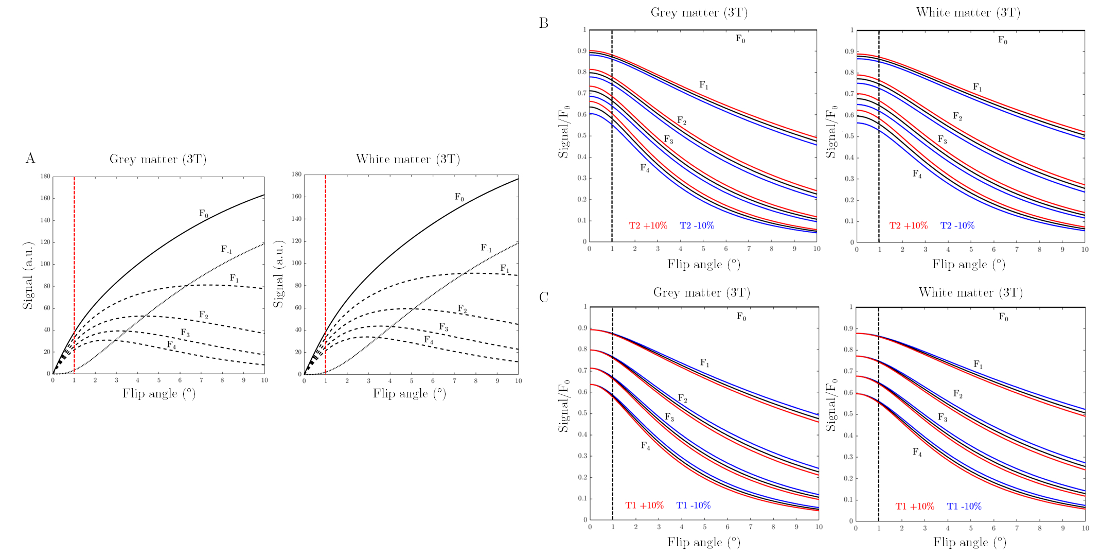
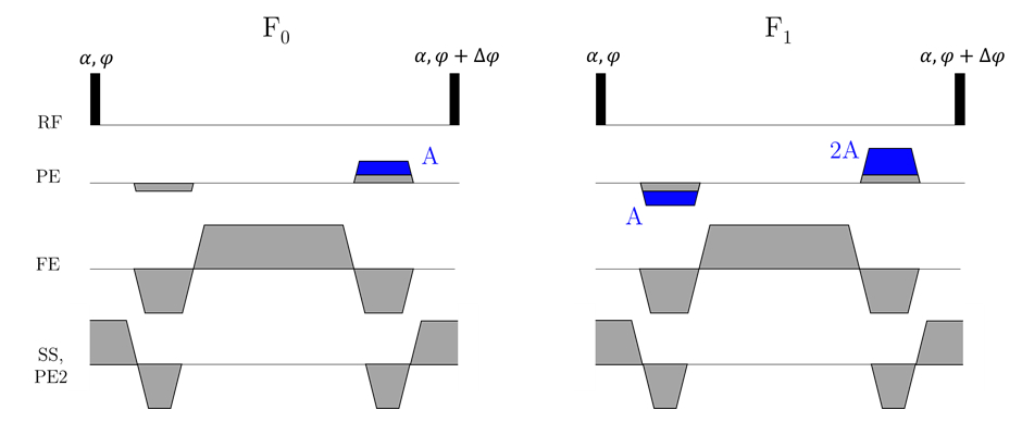
COMBINE comprises an SSFP sequence with a net unbalanced gradient in a chosen direction [1]. This enables super-resolution reconstruction, while also enabling model-based relaxometry as employed in multi-echo SSFP experiments [2]. By varying the amount of spoiling before and after the readout, we can select different configuration states (‘F-states’, signal profile in Figure 1A, pulse sequence in Figure 2) with amplitudes which are predominantly sensitive to T2 (Figure 1B) and insensitive to T1 (Figure 1C) in the low flip angle regime (α ≤ 1°).Since the gradient requirements in the super-resolution direction are greatly reduced (because we acquire low-resolution images) it is possible to reach high order F-states with only a minimal increase in the minimum TR (Figure 2). Higher order F-states have stronger T2 weighting (e.g. F4 in Figure 1B).
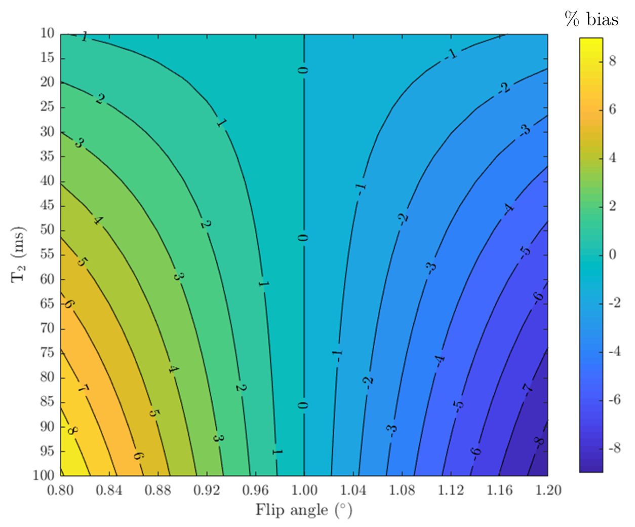
The analytical expression for the signal from each F-state is well described [2], and so from a series of two or more contrasts we can generate a T2 map, given knowledge of the flip angle (local B1+) and a rough approximation of T1. Specifically, we apply the signal equations from [2] and estimate T2 via nonlinear least squares. While T1 has minimal impact on the observed signal, variation in B1+ causes under- or overestimation of T2 (Figure 3).
Methods
We performed an experiment with the NIST/ISMRM phantom (CaliberMRI, Boulder, CO, USA) on a 3T Magnetom Prisma scanner (Siemens Healthineers, Erlangen, Germany) equipped with a 64 channel head coil. Separate T2 measurements were made with a 2D MESE sequence (TR= 3520 ms, 7 TEs= 24/48/72/96/120/144/168 ms, 0.98 x 0.98 x 5.00 mm3 voxels) and the proposed 3D T2-COMBINE approach (TR=8 ms, TE= 4 ms, α= 1°, five acquisitions of 1.0 x 5.0 x 1.0 mm3 voxels reconstructed to 1 mm isotropic, five separate acquisition contrasts: F0/F1/F2/F3/F4). A low resolution B1+ map was also acquired using the standard vendor-provided technique (tfl_b1map).MESE: A single 5mm sagittal slice was chosen at the level of the T2 contrast spheres, and each echo fitted to a monoexponential decay curve as described previously [3,4].
COMBINE: For each contrast (acquired separately to minimise TR) the total T2-COMBINE acquisition time was 5 min 20 s (including 5 shifted low-resolution images), with a field of view matching that of a sagittal whole head acquisition (250 x 250 x 160 mm3). Multi-frequency super-resolution reconstruction was performed as described previously [1]. A single 1mm sagittal slice was chosen at the level of the T2 contrast spheres, and each contrast fitted to the equations in [2] via nonlinear least squares (lsqnonlin, MATLAB, Natick, MA, USA), with a fixed T1 estimate of 1000ms and the separately obtained B1+ map. All five contrasts (F0-F4) were included in the fit.
Circular regions of interest were drawn at the centre of each sphere with equal area of 76 mm2 in-plane, and applied to each of the calculated T2 maps to calculate mean T2 estimates and standard deviations. Reference T2 values for each sphere were provided by the phantom vendor, and corrected based on in-house measurements of temperature dependence.
Results
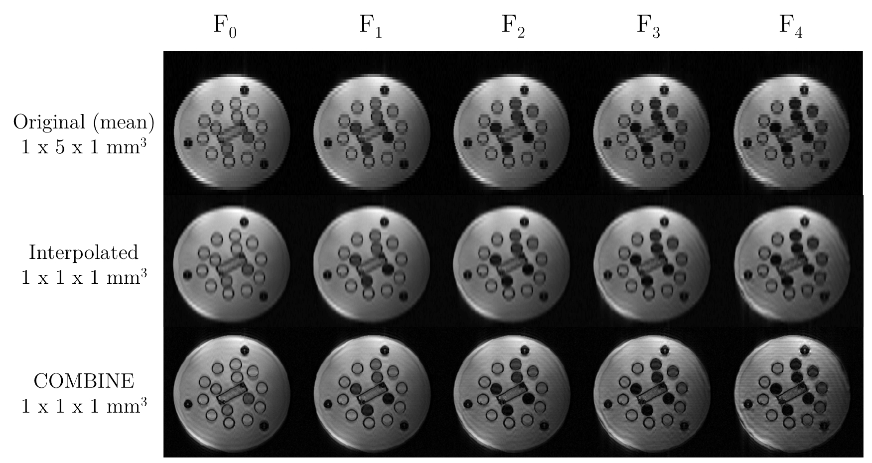
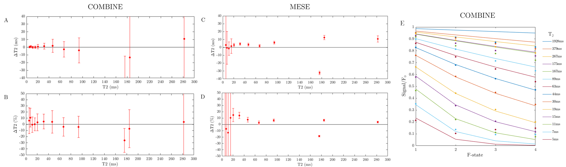
The super-resolution T2-COMBINE images are shown for each of the five contrasts in Figure 4, in comparison to the mean of the original low-resolution data. These demonstrate increasing T2 weighting with increasing F-state as predicted, despite some residual signal non-uniformities from the super-resolution reconstruction.A plot of the absolute deviation in T2 values from the reference T2 values is shown in Figure 5A for COMBINE, and in Figure 5C for MESE. This is also shown as a percentage of the reference value in Figure 5B and 5D respectively. T2 estimates from COMBINE closely match reference values in the range of T2<100ms, with increasing errors at larger T2. The larger error bars in COMBINE are in part due to the residual non-uniformities after super-resolution reconstruction. In future work we plan to develop regularised reconstruction approaches with the aim of suppressing these.
In the spheres with shortest T2 (<10ms) signal in higher F-states was affected by the noise floor, while there was a systematic underestimation of the signal in the longest T2 spheres (>100ms, Figure 5E). Despite this, the measured signal closely matches that predicted across a wide range of T2 values typically observed in vivo (Figure 5E).
Conclusion
High-resolution, low-SAR 3D T2 relaxometry is possible across a range of T2 values present in vivo using COMBINE. This provides new options for high-resolution quantitative imaging in different tissues.Acknowledgements
We wish to thank Dr Iulius Dragonu (Siemens Healthineers) for providing support for sequence development. PJL acknowledges generous funding from The Wellcome Trust (220473/Z/20/Z) and The Edmond J Safra Foundation.References
[1] Lally PJ, Matthews PM, Bangerter NK. (2020) Unbalanced SSFP for super‐resolution in MRI. Magn Reson Med. Nov 17
[2] Hänicke W, Vogel HU. (2003) An analytical solution for the SSFP signal in MRI. Magn Reson Med. Apr;49(4):771-5.
[3] Pei M et al. (2015) An Algorithm for Fast Mono-exponential Fitting Based on Auto-Regression on Linear Operations (ARLO) of Data. J Magn Reson Med. 73(2):843-850.
[4] Smith J et al. (2020) Validity and reproducibility of Magnetic Resonance Fingerprinting in the healthy human brain at 3T. Proc Intl Soc Mag Reson Med 28
[5] Zhu J et al. (2014) Relaxation Measurements in Brain tissue at field strengths between 0.35T and 9.4T. Proc Intl Soc Mag Reson Med 22Figures