Introduction

Quantitative techniques for characterizing deep learning (DL) algorithms are necessary to inform their clinical application, use, and quality assurance. Furthermore, predictions from DL models should be understood in the context of human predictions for the same clinical tasks if they are expected to assist or substitute humans in clinical decision making. A limitation of DL algorithms is their lack of generality due to the limited number of data sets available from retrospective databases. As a result, some DL algorithms are expected to make highly variable predictions on clinical tasks and therefore need to be sufficiently characterized prior to clinical use. Methods to evaluate multiple algorithms are needed to gain more insight into the variability of these algorithms. The purpose of this work was to investigate the variability of DL algorithms for contouring at a population level by training several DL algorithms for prostate and organ at risk (OAR) segmentation in prostate MRI. Each DL algorithm was treated as an independent observer of the development MRIs and predictions from populations of DL algorithms were compared with target annotations from a population of human observers performing the same task.

Methods

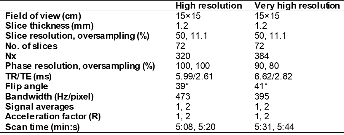
25 patients underwent low-dose-rate prostate brachytherapy (LDRPBT) and were scanned with a fully balanced SSFP pulse sequence (Table 1). A human observer study comprising 7 human analysts was conducted. The analysts included 4 radiation oncologists (ROs), 1 radiologist, 1 dosimetrist, and 1 imaging physicist, who are all involved in the treatment workflow for LDRPBT. Several techniques to minimize human observer bias were implemented in the study. The analysts contoured the prostate, external urinary sphincter (EUS), seminal vesicles (SV), rectum, and bladder in the 25 MRIs.

54 DL algorithms were successively trained on a common set of development MRIs and human segmentation masks. This yielded 54 unique DL algorithms to perform the segmentation task, each of which had unique convolution kernels and were produced as an attempt to replicate the variation in the human segmentation masks. 295 retrospectively collected 3D prostate MRIs acquired with 2 pulse sequences that yielded T2w and T2/T1w image contrast, respectively, were used for developing the DL models (250/45 training/cross validation).

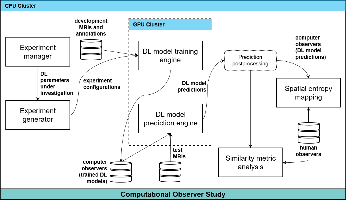
All DL experiments were performed on an NVIDIA DGX-1 workstation (Figure 1). Each of the DL models made predictions on the 25 post-implant MRIs. A 50% confidence threshold on each network’s softmax function was used to produce the binary mask of each organ from that network. Global similarity metrics were computed between the most experienced RO and all 54 DL algorithms. They were also computed amongst human observers using the most experienced RO as the reference. The similarity metrics included precision (P=TP/(TP+FP)), recall (R=TP/(TP+FN)), Dice similarity coefficient (DSC=2*P*R/(P+R)), and Matthew’s correlation coefficient (MCC=(TP*TN-FP*FN)/√((TP+FP)*(TP+FN)*(TN+FP)*(TN+FN))). Additionally, spatial distributions of the entropy of the segmentation masks were computed and compared across human and computer populations for the 25 patients. The entropy of the segmentation masks H for an observer population was computed voxel-wise; H(x,y,x)=-∑p(x_i,y_j,z_k)log(p(x_i,y_j,z_k)), where p(x_i,y_j,z_k) is the probability distribution of the tissue class of voxel (i,j,k) for the observer population. The algorithms were incorporated into a commercial treatment planning system (TPS) for visualization.

Results

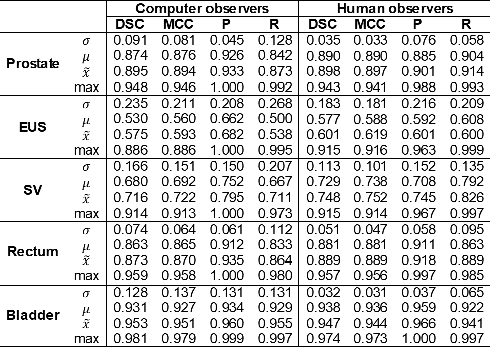
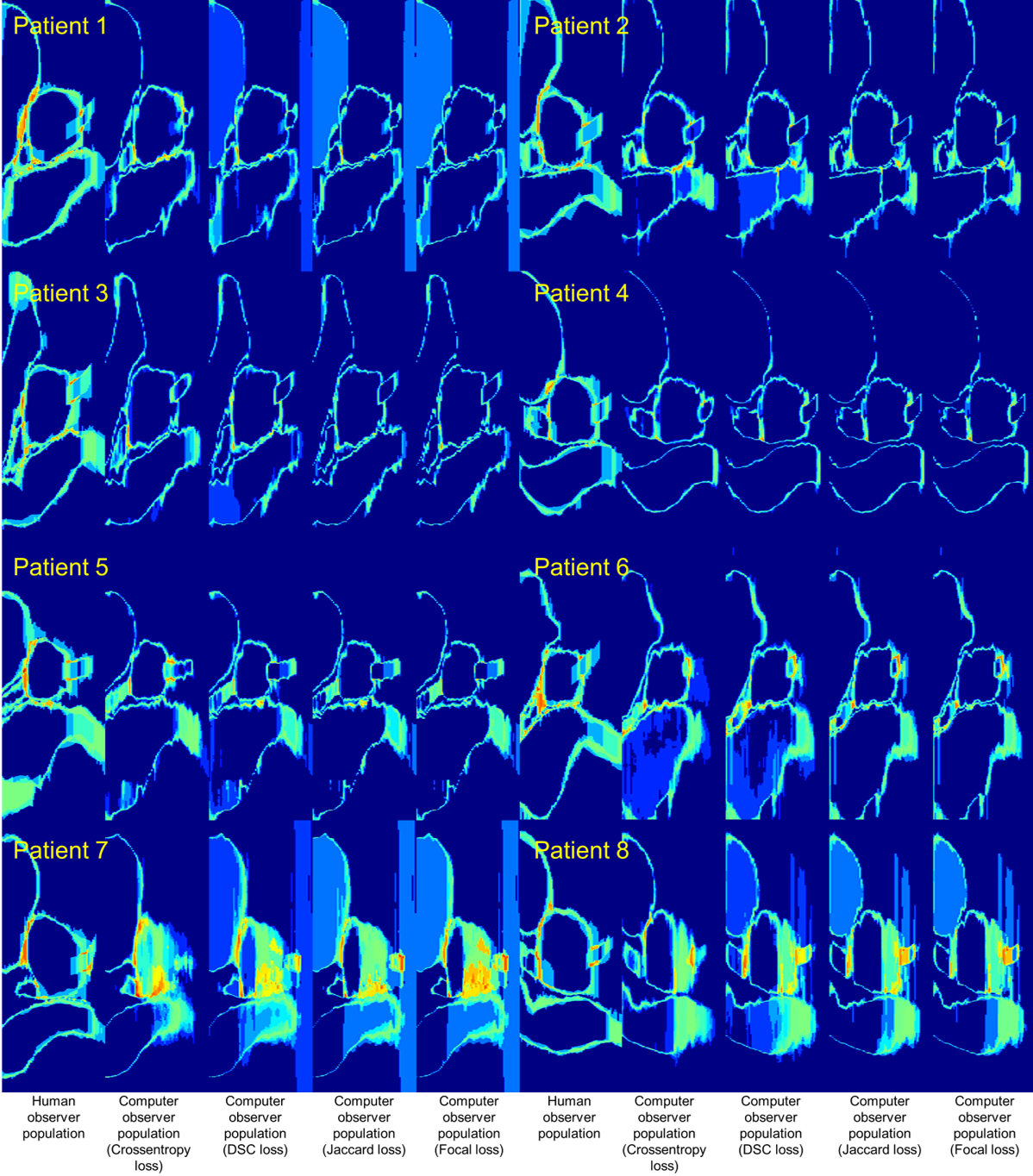
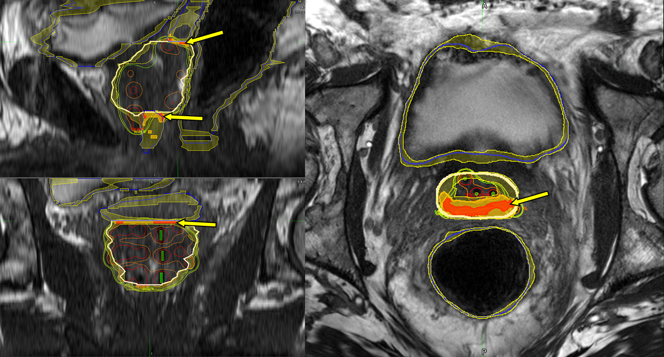
Global similarity metrics are reported in Table 2 for the experiments. Spatial entropy maps for 8 example patients compared between the human and computer observer populations revealed patterns of clustering in specific anatomic regions of the MRIs (Figure 2). The clusters with the highest entropy were located around the circumference of the target organ (prostate), especially at junctions between the target and surrounding OARs. The most common regions of high entropy clusters were observed at the bladder neck, the junction between the prostate and SV, the region along the prostate and anterior rectal wall, and the junction between the prostate apex and EUS. The computer observer population was less variable than the human observer population for some patients (e.g. Figure 2, patients 3 and 4), but was also highly variable on other patients (e.g. Figure 2, patients 7 and 8). The autocontouring predictions and spatial entropy maps computed in the TPS for one example patient (Figure 3) showed regions of high entropy clusters overlaid on their corresponding prostate MRI, providing feedback on anatomical regions of high variability in contouring for review and refinement.

Discussion/Conclusions

Global similarity metrics are commonly used to characterize the performance of DL algorithms for segmentation tasks. However, these metrics are limited in that they do not provide information about local segmentation performance. Moreover, the clinical context for these metrics is often absent in reporting of segmentation algorithms (e.g. what does a prostate DSC of 0.87 really mean?). This work attempts to help address these questions for the task of prostate and OAR segmentation in prostate MRI. We compared four global similarity metrics between human and computer observer populations to provide context on the numerical values of these metrics. We also presented spatial entropy mapping case studies for 8 example patients, demonstrating that populations of DL algorithms produced patterns of lower, similar, and higher spatial entropy of tissue classes as compared to a group of analysts involved in LDRPBT clinical workflow. These findings have several potential implications for the use of autocontouring algorithms for MRI-based LDRPBT.

Acknowledgements

No acknowledgement found.