Introduction

Multi-parametric MRI is used for the characterisation of suspected localised prostate cancer and includes diffusion weighted imaging and a T2 weighted image with a single effective echo time. Using multiple-echo sequences, additional information about tissue T2 can be obtained from the decay of the signal with echo time and quantified using the luminal water fraction (LWF). With increasing Gleason grade, the luminal space decreases and hence the luminal contribution to the MR signal decreases. Tissue with a long T2, above a threshold of 200ms, is classified as luminal. LWF is then the ratio of the amount of long T2 tissue to the total (amount of long plus short T2 tissue). The LWF has been shown to correlate with histological Gleason grade and radiologist scoring^1-3 . The multi-echo sequence benefits from low distortions compared to EPI-based diffusion imaging.

For each tissue component, the signal decreases exponentially with echo time at a rate determined by the T2 of the component. The measured signal from each voxel is the sum of exponentials from all tissue components within that voxel. The fitting process attempts to determine the amount of each tissue type present – the T2 distribution. Fitting the parameters of the distribution can be slow, sensitive to starting estimates and many parameter values may give similar fits. In essence, the LWF quantifies the ratio of signal that persists at long echo times, to the overall signal. This suggests two simpler alternatives; the average signal from the later echo times (normalised by the overall median signal), and, fitting the amplitudes of a bi-exponential distribution with a fixed long and short T2.

Methods

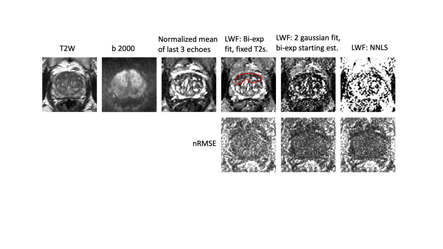
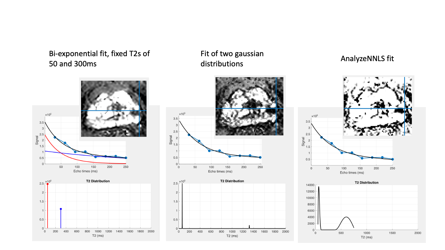
Representative datasets were selected retrospectively from an ongoing study⁴ for which patients had provided written consent. Scans were acquired on a Philips 3T Achieva and included an axial T2 weighted sequence, a diffusion weighted sequence (b-value 2000) and a multi-echo sequence (8 echoes each separated by 31.25ms, 1.5x1.5mm in-plane resolution, 17 slices 4mm thick covering the entire prostate).

Four fits were compared. A) The mean signal from the last three echoes (at 188, 219 and 250ms), normalised by the median signal from the first echo over the entire volume. B) LWF computed from a bi-exponential fit with fixed T2s of 50ms (short) and 300ms (long). The fit was implemented in MATLAB as the solution of a linear system with 8 equations and 2 unknowns (the amplitudes of the short and long T2 components). Using the mldivide function, the entire volume can be fit non-iteratively. C) LWF calculated from a probability distribution using two gaussian probabilities using the result from B) as a starting estimate. This fit uses the MATLAB lsqnonlin to find the unknown amplitudes, means and standard deviations for a short and long T2 gaussian distribution. D) LWF computed from a distribution calculated using AnalyzeNNLS⁵. The Root Mean Square Error normalized to the first echo signal was also calculated (nRMSE).

Results and Discussion

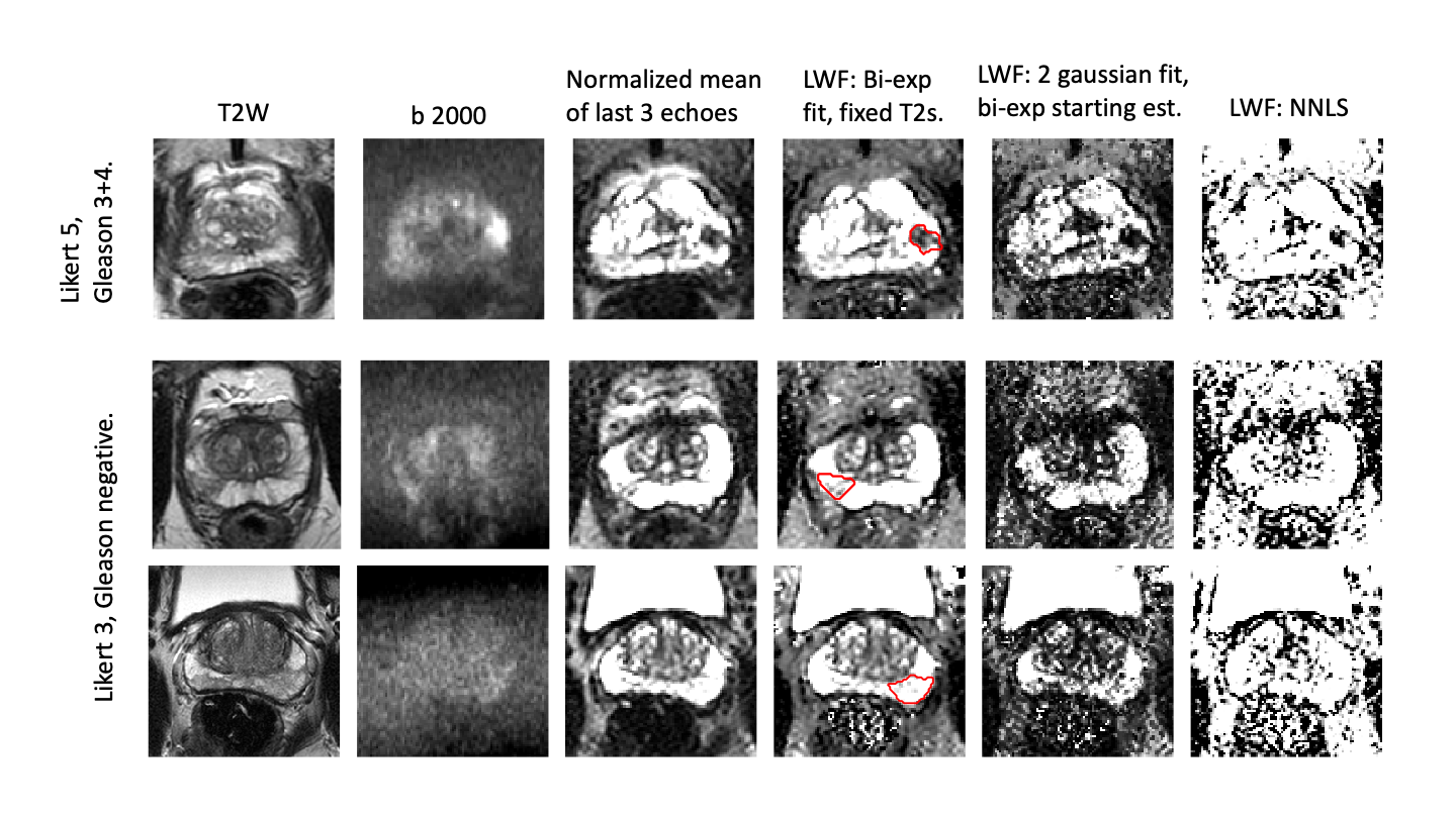
The times for calculation of the mean signal from the last 3 echoes and the bi-exponential fit with fixed T2s are near instantaneous for an entire volume, whereas iterative fits C) and D) take around a minute for a cropped region of a single slice.

Fig 1 shows T2, diffusion and LWF fits and corresponding nRMSE error maps. The fits with more parameters are able to fit the data more closely (lower fit error) and all fits show broadly uniform error distribution across the prostate. The lesion (outlined in red) is visible in all fits. Fig 2 shows the fitted distributions for a sample voxel, highlighting how different parameters can yield similar fits to the data . Fig 3 shows example LWF maps from other patients. Visual analysis of sample LWF datasets suggests a differing appearance of noise-like features between the different fits, but no consistent differences in lesion conspicuity. Further analysis will be required to determine thresholds for disease and to assess conspicuity across larger numbers of patients.

In summary, fitting of multi-exponentials is a poorly determined problem with many fit parameter values giving similar fits to the measured signal. The LWF metric mitigates wide variations in fit parameters by providing a single summary metric. Simpler non-iterative fits that are near instant might be useful on their own, or as a starting estimate for refinement by iterative fits. Further work is needed to assess the impact on lesion conspicuity and clinical efficacy.

Acknowledgements

This work was undertaken at UCLH/UCL, which receives funding from the UK Department of Health’s the National Institute for Health Research (NIHR) Biomedical Research Centre (BRC) funding scheme. This work was also supported by the Medical Research Council and Cancer Research UK.