4051
Deep CNNs with Physical Constraints for simultaneous Multi-tissue Segmentation and Quantification (MSQ-Net) of Knee from UTE MRIs
Xing Lu1, Yajun Ma1, Saeed Jerban1, Hyungseok Jang1, Yanping Xue1, Xiaodong Zhang1, Mei Wu1, Amilcare Gentili1,2, Chun-nan Hsu3, Eric Y Chang1,2, and Jiang Du1
1Department of Radiology, University of California, San Diego, San Diego, CA, United States, 2Radiology Service, Veterans Affairs San Diego Healthcare System, San Diego, CA, United States, 3Department of Neurosciences, University of California, San Diego, San Diego, CA, United States
1Department of Radiology, University of California, San Diego, San Diego, CA, United States, 2Radiology Service, Veterans Affairs San Diego Healthcare System, San Diego, CA, United States, 3Department of Neurosciences, University of California, San Diego, San Diego, CA, United States
Synopsis
In this study, we proposed end-to-end deep learning convolutional neural networks to perform simultaneous segmentation and quantification (MSQ-Net) on the knee without and with physical constraint networks (pcMSQ-Net). Both networks were trained and tested for the feasibility of simultaneous segmentation and quantitative evaluation of multiple knee joint tissues from 3D ultrashort echo time (UTE) magnetic resonance imaging. Results demonstrated the potential of MSQ-Net and pcMSQ-Net for fast and accurate UTE-MRI analysis of the knee, a “whole-organ” approach which is impossible with conventional clinical MRI.
Introduction
Compared with qualitative magnetic resonance imaging (MRI), quantitative MRI is a more accurate approach in evaluating underlying pathology and disease course. However, the physical model-based voxel-fitting quantification process is normally quite slow and not robust. Even worse, when there are multiple tissues in the area of interest, such as in the knee where articular cartilage, menisci, ligaments, and many other tissues all contribute to joint function and degeneration, it is even more time-consuming to perform second-stage analysis of different tissues. It would be of great clinical values to simultaneously segment and quantify all major knee joint tissues accurately and effectively.Deep Convolutional Neural Networks (DCNN) have been shown as a feasible method for accurate segmentation of multiple organs in medical imaging analysis2,3. Recently, there has been intense interest in employing DCNN models to obtain quantitative mapping of MRI parameters in a faster way, with and without physical constraints4,5.
In this study, two end-to-end DCNNs of Simultaneous Segmentation and Quantification (MSQ-Net) and MSQ-Net with physical constraints (pcMSQ-Net) were proposed to segment and quantify different tissue components simultaneously in the knee joint.
Methods
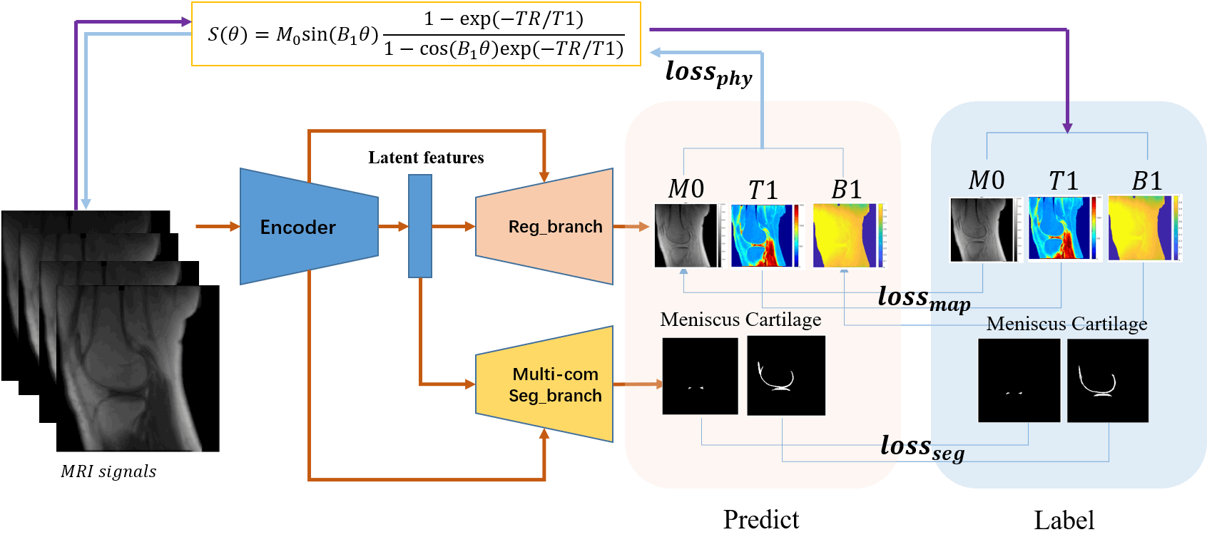
The MSQ-Net network is based on a U-Net style DCNN but with two branches for outputs, named Reg_branch and Seg_branch (Figure 1). Along the encoder path, down-samplings are applied to enable subsequent feature extractions at coarser scales. Latent features are shared for both up-sampling branches, and up-samplings are conducted to support subsequent feature extractions at finer scales. Between convolutional blocks, skip connections are established. For Reg_branch, quantitative MRI parameter maps are generated according to the voxel-fitting-based maps as the ground truth (GT), with l1 loss (lossmap ) as the constraint. For Seg_branch, the meniscus and cartilage masks are generated with binary cross entropy loss and dice loss-based segmentation loss (lossseg). For MSQ-Net, the total loss (lossMSQ) consists of lossmap and lossseg(1-3).$$loss_{MSQ}=\lambda_1loss_{map}+\lambda_2loss_{seg} (1)$$
$$loss_{seg}=\lambda loss_{bce}+(1-\lambda)loss_{dice} (2)$$
$$loss_{map}=l1(Y,\widehat{Y}),Y=[M0,T1,B1] (3)$$
A physical-constraint loss (lossphy) is applied to feed the predicted maps back to generate the input MRI signals with different flip angles ($$$\theta$$$). MSQ-Net with lossphy is named as pcMSQ-Net, which has a total loss of losspcMSQ(4-6).
$$loss_{pcMSQ}=\lambda_1loss_{map}+\lambda_2loss_{seg}+\lambda_3loss_{phy} (4)$$
$$loss_{phy}=l1(S,\widehat{S}) (5)$$
$$S=M_0sin(B_1\theta)\frac{1-exp(T_R/T_1)}{1-cos(B_1\theta)exp(-TR/T_1)} (6)$$
We validated the method through T1 mapping of both articular cartilage and menisci in the knee joint with Ultrashort Echo(UTE) MRIs(as UTE techniques can be applied to all the principal knee joint tissues, which may otherwise be “invisible” with conventional clinical scans). For every subject, a series of T1-weighted images was acquired using a 3D UTE sequence with variable flip angles (VFA). Three-dimensional spiral sampling was performed with conical view ordering using a very short echo time (TE) of 32 µs, repetition time (TR) of 20 ms, and VFAs of 5°, 10°, 20°, and 30°. Subsequently, image registration was performed to minimize inter-scan motion. M0, T1, and B1 maps were derived via non-linear fitting using the Levenberg‐Marquardt algorithm6,7.
A total of 720 slice images from 30 subjects (including healthy volunteers and patients with different degrees of osteoarthritis (OA)) was used for model training, and 96 images of four additional subjects was used for model testing. The DCNNs were implemented with pytorch 1.1.0 on a workstation with a Nvidia GTX 1080 Ti (11 GB GPU memory). Both MSQ-Net and pcMSQ-Net were trained with the same datasets and hyper-parameters, such as learning rate from 0.001 with a cosine-annealing strategy, and epochs of 500. To evaluate the performance of T1 mapping for both DCNN models, a ssim score was applied8. Models with the highest ssim scores during training were saved for further evaluation.
Results and Discussion
Figure 2 shows typical results for the outputs of the MSQ-Net and pcMSQ-Net, demonstrating that both MSQ-Net and pcMSQ-Net have the ability to simultaneously generate reasonable parameter maps, as well as segmentation masks. As shown in Figure 2 (b) and (c), Red and yellow arrows indicate pcMSQ-Net produced better details in T1 maps. In Figure(d), the cartilage masks generated by DCNNs are slightly different from radiologist-labeled masks, as depicted with green arrows. This discrepancy can be improved in the future by including more datasets for training and by making further improvements to the model itself.Comparison of metrics results can be found in Table 1. pcMSQ-Net has better metrics compared to MSQ-Net. pcMSQ-Net obtained a mean ssim score of 0.925 for the test dataset, superior to the MSQ-Net of 0.854.
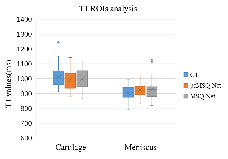
Region of interest (ROI) analysis based on the T1 maps and masks generated from both models was applied to test datasets with comparison to the GT based on labelling by experienced radiologists. Figure 3 shows that both MSQ-Net and pcMSQ-Net have similar results compared with the GT. Statistical results of the ROI analysis of the GT, MSQ-Net, and pcMSQ-Net are summarized in Table 2. Limited number of subjects in test datasets and potential fat contamination due to partial volume artifact may lead to reduced T1s, especially for articular cartilage.
Conclusion
In this study, two DCNN models, MSQ-Net and pcMSQ-Net, were proposed for simultaneous segmentation and T1 quantitative mapping of multiple knee joint tissues, including the cartilage and meniscus. Compared to MSQ-Net, pcMSQ-Net obtained better image quality. Both models obtained reasonable ROI analysis results compared with results by experienced radiologists.Acknowledgements
The authors acknowledge grant support from NIH (R01 AR068987, R01AR075825), and Veterans Affairs (I01RX002604 and I01CX001388) and GE Healthcare.References
1. Ricardo de Mello, Yajun Ma, Yang Ji, Jiang Du, and Eric Y. Chang. Quantitative MRI Musculoskeletal Techniques: An Update. American Journal of Roentgenology 2019 213:3, 524-533 2. Ronneberger O., Fischer P., Brox T. U-Net: Convolutional Networks for Biomedical Image Segmentation. MICCAI 2015. 3. Hesamian, M.H., Jia, W., He, X. et al. Deep Learning Techniques for Medical Image Segmentation: Achievements and Challenges. J Digit Imaging 32, 582–596 (2019). 4. Liu, F, Feng, L, Kijowski, R. MANTIS: Model‐Augmented Neural neTwork with Incoherent k‐space Sampling for efficient MR parameter mapping. Magn Reson Med. 2019; 82: 174– 188. 5. Yoon J, Gong E, Chatnuntawech I, Bilgic B, Lee J, Jung W, Ko J, Jung H, Setsompop K, Zaharchuk G, Kim EY, Pauly J, Lee J. Quantitative susceptibility mapping using deep neural network: QSMnet. Neuroimage. 2018 Oct 1;179:199-206. 6. Ma YJ, Lu X, Carl M, Zhu Y, Szeverenyi NM, Bydder GM, Chang EY, Du J. Accurate T1 mapping of short T2 tissues using a three-dimensional ultrashort echo time cones actual flip angle imaging-variable repetition time (3D UTE-Cones AFI-VTR) method. Magn Reson Med. 2018 Aug;80(2):598-608. 7. Ma YJ, Zhao W, Wan L, Guo T, Searleman A, Jang H, Chang EY, Du J. Whole knee joint T1 values measured in vivo at 3T by combined 3D ultrashort echo time cones actual flip angle and variable flip angle methods. Magn Reson Med. 2019 Mar;81(3):1634-1644. 8. Z. Wang, A. C. Bovik, H. R. Sheikh and E. P. Simoncelli, Image quality assessment: From error visibility to structural similarity, IEEE Transactions on Image Processing, vol. 13, no. 4, pp. 600-612, Apr. 2004.Figures
Figure
1. Network architecture of MSQ-Net and pcMSQ-Net. MSQ-Net with lossphy
to feed back the maps predicted from the model to the input MRI signals,
according to equation (6), named physical constraint MSQ-Net (pcMSQ-Net).
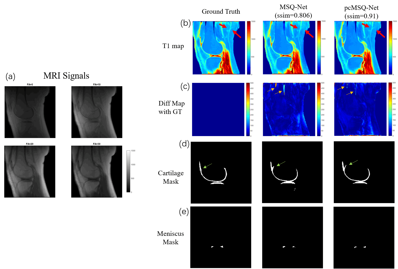
Figure 2. Typical results for MSQ-Net and pcMSQ-Net.(a)
MRI input signals with different Flip Angles(FAs); (b). T1 maps of GT, and
predicted by MSQ-Net, pcMSQ-Net; (c). Difference map from GT. Yellow arrows
demonstrates obvious errors could be found in MSQ-Net in some low-signal area
while not shown in pcMSQ-Net. (d) and (e), masks of cartilage and meniscus
of GT, and predicted by MSQ-Net and pcMSQ-Net.
Figure
3. T1 ROIs analysis for cartilage and meniscus with ground truth(GT), MSQ-Net and pcMSQ-Net.
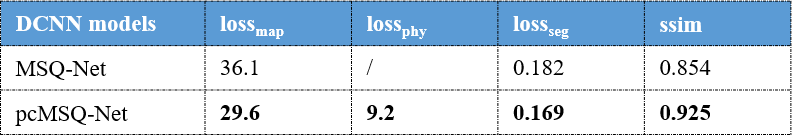
Table 1. Evaluation metrics for both MSQ-Net and pcMSQ-Net.
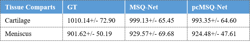
Table 2. Statistical results for the ROI analysis based on GT, MSQ-Net and pcMSQ-Net.