4039
B0-shimming methodology for affordable, compact, and homogeneous low-field MR magnets1Physikalisch-Technische Bundesanstalt (PTB), Braunschweig and Berlin, Germany, 2Leiden University Medical Center (LUMC), Leiden, Netherlands
Synopsis
In this work, B0-shimming techniques are investigated allowing the construction of simple, low-cost, and homogeneous Halbach-based low-field MR magnets. The techniques are applied to build a desktop MR magnet at B0=0.1T and can be easily scaled to magnet designs of larger diameter. The presented shimming approach improved B0 homogeneity by a factor of ~8 from 5448ppm to 682ppm in a 2D target region. All design files and code concerning this work will be made available open source on www.opensourceimaging.org.
Introduction
Low-field MRI is showing an increased interest by the MR community.1-2 The advantages of lower fields, such as safety or improved imaging contrasts, alongside the chance of giving many more patients worldwide access to affordable diagnostic imaging, are driving innovations.3-4 The use of small rare-earth magnets enables designs of small and lightweight low-field MR magnets, reducing the overall costs of an MR system drastically.5-10 A major challenge of these designs is to achieve the targeted B0 field distribution since tiny variations in remanence, magnetization direction, production tolerances or placement of the individual magnets lead to substantial differences between simulated and constructed fields.In this work, B0-shimming techniques are investigated allowing to construct simple, low-cost, and homogeneous Halbach-based MR magnets. These techniques are applied to build a desktop MR magnet at B0=0.1T and they can be easily scaled to bigger magnet designs.
Methods
Magnet assemblyThe magnet design target is a low-cost (<2000€), lightweight (<15kg) and small (370x340x250)mm3 desktop MR magnet with a targeted inner bore diameter of 10cm (including gradient coils), a spherical FoV of 4cm in diameter, and a field strength of B0=0.1T.
The core of the magnet consists of three rings (denoted as “rings 1-3”) with 40 octagonal (width: 14mm, circumradius: 11.64mm, NdFeB, N50, Br=1.43T) magnets per ring in Halbach arrangement (Fig.1a). All magnets are enclosed in selective laser sintered polyamide (SLS) holders. Rings 1-3 are mounted on threaded brass rods with brass nuts.
In between these rings, shim inserts using cubic (9mm, NdFeB, N42, Br=1.3T) magnets are placed (Fig.1b-f). The final magnet is shown in Fig.1g. The shim magnets are enclosed in SLS holders, which can be inserted without modification of the core magnet assembly, allowing to iteratively place various shims if needed. All designs were modelled with the open source software FreeCAD v0.18.
B0-shimming
After construction and adjustment of rings 1-3, the field is measured with a Hall sensor (LakeShore Cryotronics, Westerville, Ohio, USA) and the open source 3-axis positioning system COSI Measure.11
A genetic algorithm was used to determine the magnet size for the shim magnets, their placement and orientation (0°, 90°,180°, 270°) deviating from a radial arrangement (k=1).9 The z-component of the magnetic flux distribution of each shim magnet is calculated with the dipole approximation from the magnetic moment.12 All fields are pre-calculated for each magnet and orientation. 25000 random shim placements are evolved for a minimum of 300 iterations until the last 20% of the iterations do not improve. The evolution was executed with tournament selection comparing three randomly picked individuals, two-point crossover with 75% probability, and mutation with 20% probability, where every individual magnet is rotated or omitted with 5 % probability.
The target field approach (TF) and spherical harmonics (SH) were used and compared for the shimming procedure. The cost function for the TF is the peak-to-peak amplitude in a 2D slice, while for the SH approach, it is calculated by the sum of the SH coefficients (greater than 0) in a 3D sphere, both regions of 4cm in diameter.
Results
The SH series shows that the parameters representing the field can be truncated to 19 (from 1600 measurement points), while still reflecting the measured field distribution accurately (Fig.2). This decreases the calculation time by a factor of 3 compared to using the TF approach. Using SH also allows to decrease the measurement time for field mapping, which can be used at a later stage to iteratively improve B0-field homogeneity. The shim magnet size that was determined by the genetic algorithm found an optimum for 9 mm cubic magnets, which were then used for the shim (Fig.3).2D-TF
The initial B0 field homogeneity of 5448ppm was improved by a factor ~8 to 682ppm, which is close to the predicted field homogeneity by the genetic algorithm of 560ppm over that region (Fig.4).
3D-SH
The B0 field homogeneity for the sphere was 8271ppm, which could be improved by a factor of 2.2 to 3759ppm applying B0 shimming (Fig.5). The predicted value was 2596ppm and the main contributor to the inhomogeneities was the SH coefficient of the fourth degree, which could not be shimmed efficiently using the current setup. The implementation of a shim with the TF on the same region resulted in 3932ppm, revealing no drawback by the applied truncation of the SH.
Discussion and Conclusion
A low-cost and small low-field desktop MR magnet (B0=0.1T) including a simple shimming method is presented. Both the magnet and the shim can be assembled easily with minimal tools needed. The genetic algorithm and the B0-shim methodology were able to improve B0-homogeneity substantially by a factor of 8 to 682ppm in a 2D slice. For a 3D shimming target, different shim arrangements need to be investigated in order to improve the homogeneity further. The proposed method is scalable to other Halbach-based MR magnets and provides a good basis for a second stage B0-shimming based on, e.g. shim coils. The method is expected to perform better for bigger MR magnets, where errors e.g. from individual magnet placement are less severe. All design files and code concerning this work will be made available open source on www.opensourceimaging.org.Acknowledgements
No acknowledgement found.References
1. Marques JP, Simonis FFJ, Webb AG. Low-field MRI: An MR physics perspective. Journal of Magnetic Resonance Imaging 2019;49:1528–1542 doi: 10.1002/jmri.26637.
2. Wald LL, McDaniel PC, Witzel T, Stockmann JP, Cooley CZ. Low-cost and portable MRI. Journal of Magnetic Resonance Imaging 2020;52:686–696 doi: 10.1002/jmri.26942.
3. Campbell-Washburn AE, Ramasawmy R, Restivo MC, et al. Opportunities in Interventional and Diagnostic Imaging by Using High-performance Low-Field-Strength MRI. Radiology 2019:190452 doi: 10.1148/radiol.2019190452.
4. Winter L, Pellicer-Guridi R, Broche L, et al. Open Source Medical Devices for Innovation, Education and Global Health: Case Study of Open Source Magnetic Resonance Imaging. In: Co-Creation. Springer; 2019. pp. 147–163.
5. Blümler P, Casanova F. CHAPTER 5. Hardware Developments: Halbach Magnet Arrays. In: Johns ML, Fridjonsson EO, Vogt SJ, Haber A, editors. New Developments in NMR. Cambridge: Royal Society of Chemistry; 2015. pp. 133–157. doi: 10.1039/9781782628095-00133.
6. Cooley CZ, Stockmann JP, Armstrong BD, et al. Two-dimensional imaging in a lightweight portable MRI scanner without gradient coils. Magnetic Resonance in Medicine 2015;73:872–883 doi: https://doi.org/10.1002/mrm.25147.
7. Cooley CZ, Haskell MW, Cauley SF, et al. Design of Sparse Halbach Magnet Arrays for Portable MRI Using a Genetic Algorithm. IEEE Transactions on Magnetics 2018;54:1–12 doi: 10.1109/TMAG.2017.2751001.
8. McDaniel PC, Cooley CZ, Stockmann JP, Wald LL. The MR Cap: A single-sided MRI system designed for potential point-of-care limited field-of-view brain imaging. Magnetic Resonance in Medicine 2019;82:1946–1960 doi: https://doi.org/10.1002/mrm.27861.
9. O’Reilly T, Teeuwisse WM, Webb AG. Three-dimensional MRI in a homogenous 27 cm diameter bore Halbach array magnet. Journal of Magnetic Resonance 2019;307:106578 doi: 10.1016/j.jmr.2019.106578.
10. Winter L, Barghoorn A, Blümler P, Niendorf T. COSI Magnet: Halbach magnet and Halbach gradient designs for open source low cost MRI. In: Proc Intl Soc Mag Reson Med. ; 2016. p. 3568.
11. Han H, Moritz R, Oberacker E, Waiczies H, Niendorf T, Winter L. Open source 3D multipurpose measurement system with submillimetre fidelity and first application in magnetic resonance. Scientific reports 2017;7:13452.
12. Jackson JD. Classical Electrodynamics. 3rd ed. Berkley: John Wiley & Sons, Inc.; 1998.
Figures
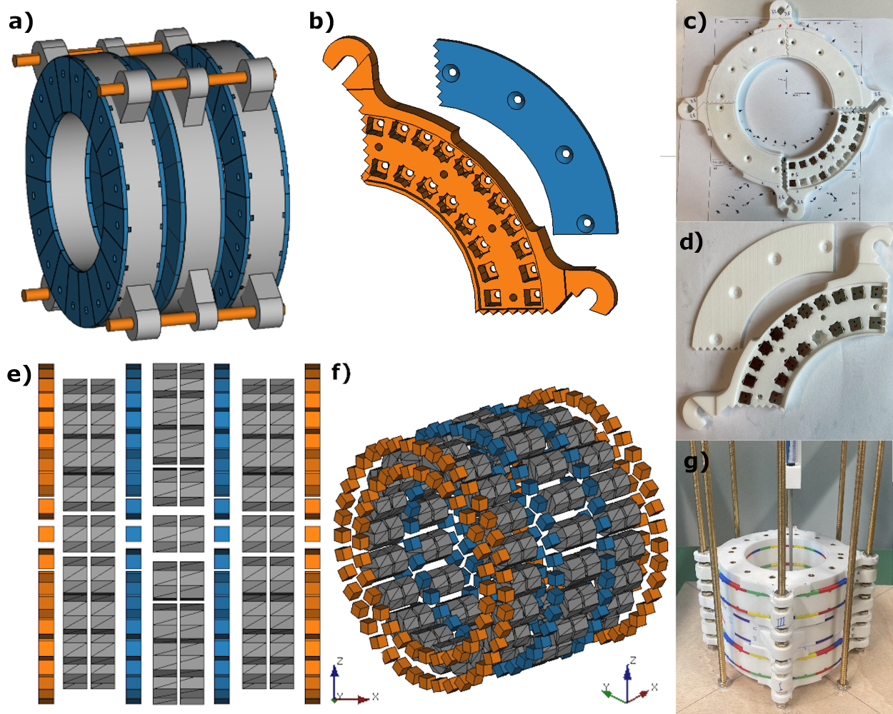
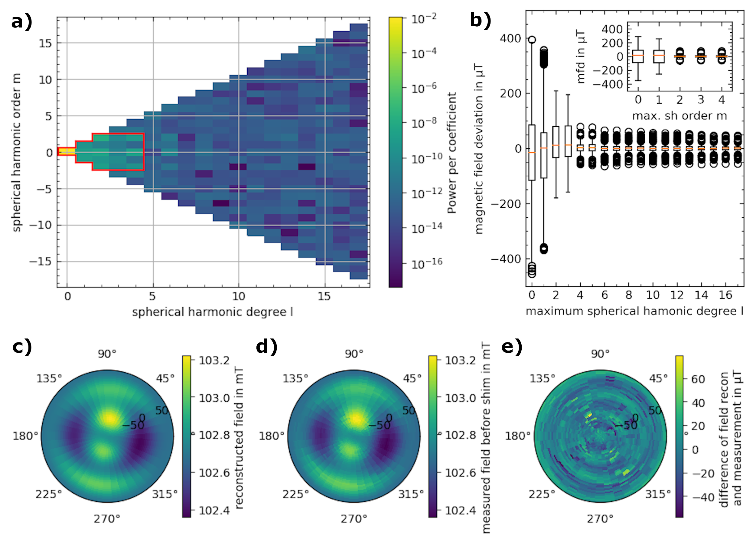
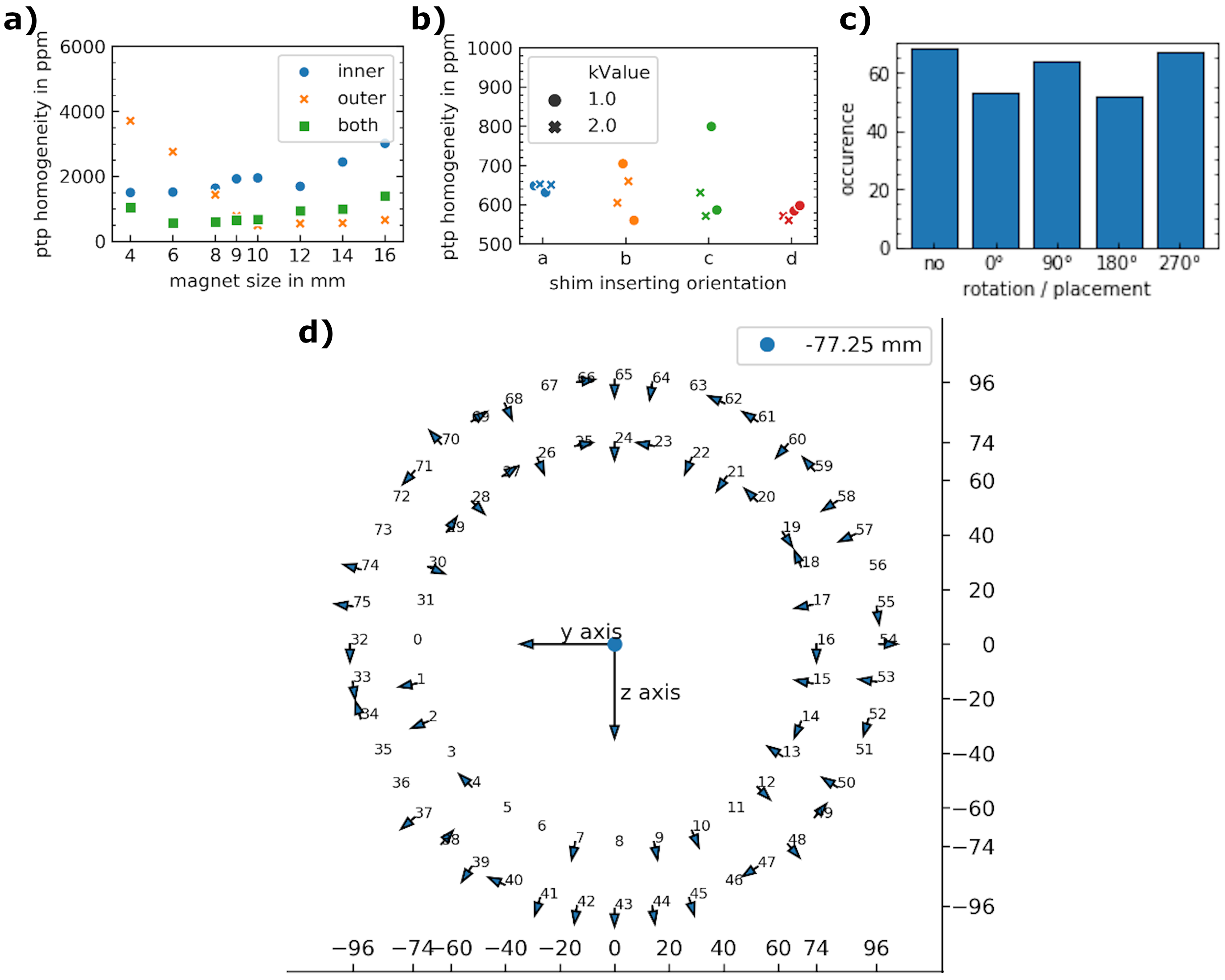
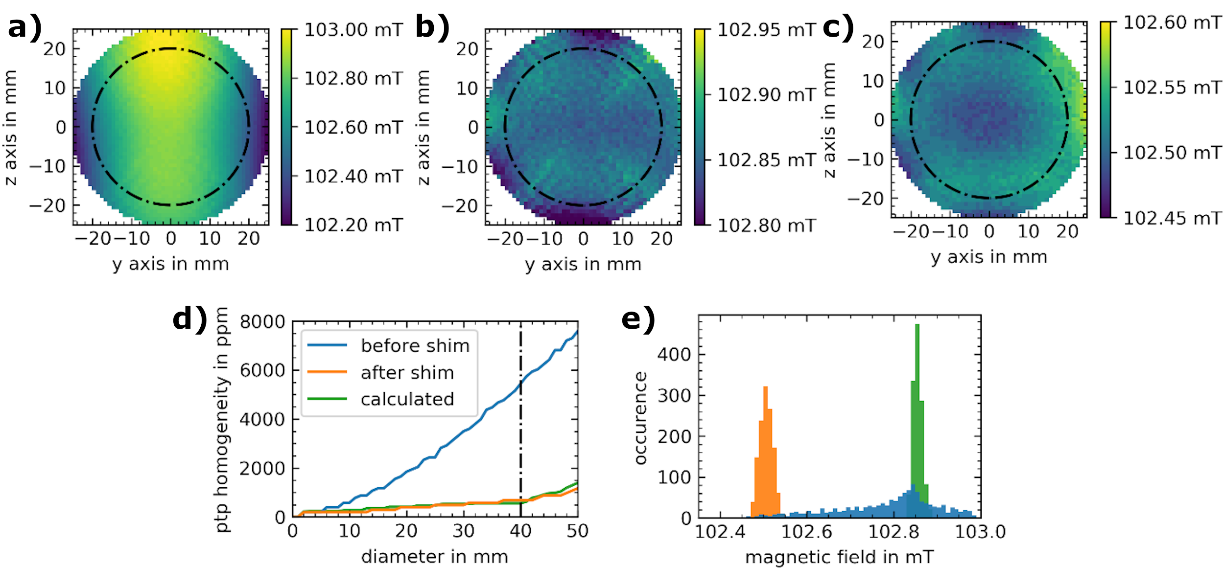
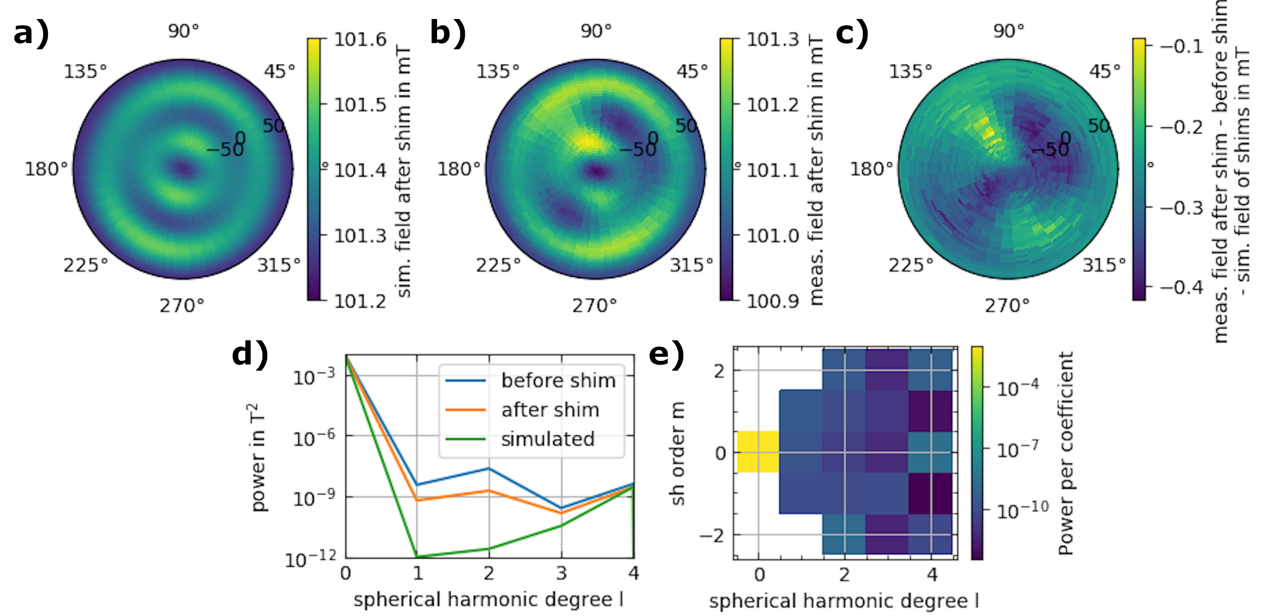
Figure 5: a) Calculated and b) measured magnetic field B0 after the 3D-SH shim. c) Difference between b) and a). The color-scales in a) and b) are shifted by 0.3 mT, conserving the absolute range. d) Power of SH degree in the unshimmed desktop magnet (blue), determined in simulations by the shimming algorithm (green) and measured after the shim placement (orange). e) SH coefficients of the measured field after shimming.