Introduction

Proton MR spectroscopy has shown promising evidence to assess cardiac metabolism¹. At the moment this is commonly performed at 1.5T or 3T. Higher field strengths have the advantage of higher thermal polarization and a larger peak separation for spectroscopy. This comes, however, at the expense of larger field inhomogeneities, higher SAR levels and increased ECG interference. Lower field strengths can benefit from lower SAR levels and therefore shorter RF pulse lengths and echo times², which can together with increased T₂ and decreased T₁ values^3–5 lead to an increase in signal. A more homogeneous field and therefore higher T₂^* values might compensate for the decrease in spectral separation at lower fields.
The aim of the present work was to investigate the feasibility of ¹H-MRS for the assessment of triglyceride levels in human calf muscle and myocardium at a custom 0.75T scanner and compare this to measurements at 1.5T and 3T.

Methods

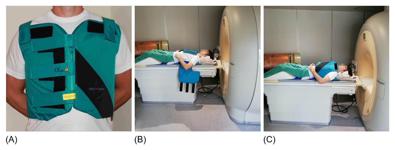
A 3T Achieva scanner (Philips Healthcare, Best, the Netherlands) was ramped down to a field strength of 0.75T. A custom-made 4-channel transmit/receive coil array (Clinical MR Solutions, Shadybrook, WI, USA) (Figure 1), which was originally made to sample on the ¹³C frequency at 3T, was tuned to the ¹H frequency at 0.75T. Reference measurements were performed at both a 1.5T Philips Achieva scanner using a five-channel cardiac receiver array and at another 3T Philips Achieva scanner using a two-channel Flex-L coil.
Measurements were performed in both the calf muscle and the interventricular septum of 3 healthy volunteers. Spectra were acquired with a voxel size of 10×20×40 mm³; pencil-beam volume shimming and local power optimization⁶ were performed prior. TE ranged from 15 ms at 0.75T to 26 ms at 3T with a TR of 2000 ms. CHESS based water suppression was performed; the number of water-suppressed averages was 96 for calf muscle and 192 for myocardium. Spectral bandwidth in the leg was 1000 Hz, 2000 Hz and 4000 Hz at 0.75T, 1.5T and 3T respectively, and 2000 Hz in the heart for all field strengths (1024 samples). Cardiac measurements were ECG-triggered to end systole and respiratory gating was applied (window = 4 mm). Scan times were identical at all field strengths. Additionally, series with different echo times (range = 15-400 ms, 11 steps) and repetition times (range = 375-5000 ms, 9 steps) were acquired for the water-unsuppressed signal (NSA = 16) of the calf muscle.
All spectra were reconstructed in MATLAB using a customized reconstruction pipeline. Spectra were fitted with Lorentzian line shapes in the time-domain using AMARES (jMRUI, version 5.2)⁷. T₁ was acquired by fitting the data from the TR series according to $$$M_z=M_0\left(1-c\left(e^{-\frac{TR}{T_1}}\right)\right)$$$, the TE series were fitted with $$$M_{xy}=M_0\left(e^{-\frac{TE}{T_2}}\right)$$$ and T₂^* was calculated based on linewidth of the water peaks according to $$$fwhm=\frac{1}{\pi T_{2}^{*}}$$$. T₁, T₂ and T₂^* were fitted as a function of magnetic field according to $$$T=a\left(B_0\right)^b$$$. Spectra consisting of TMA, CR, TG-CH₂- and TG-CH₃ were simulated using Bloch equations for field strengths of 0.75T, 1.5T and 3T. Realistic metabolite SNR values were assumed for 1.5T; SNR at 0.75T and 3T was calculated based on these values and an SNR simulation based on first principles. ΔB₀ was calculated for each field strength based on the measured T₂^* of water in the septum; this was used to calculate T₂^* values of the separate metabolites and define linewidths.

Results

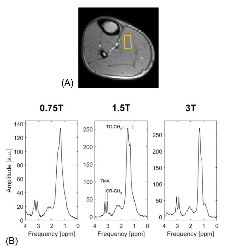
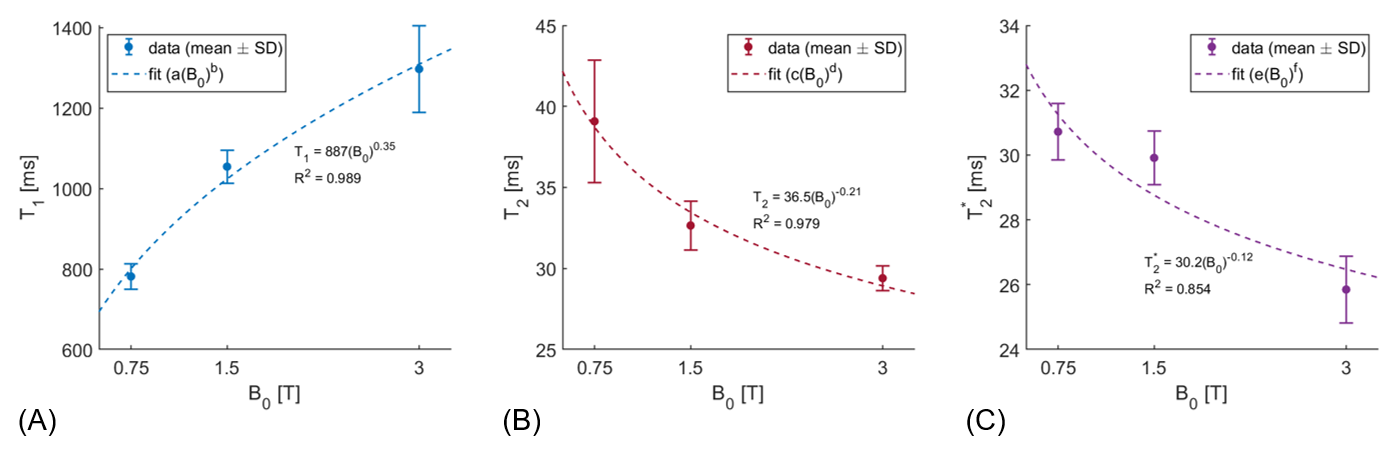
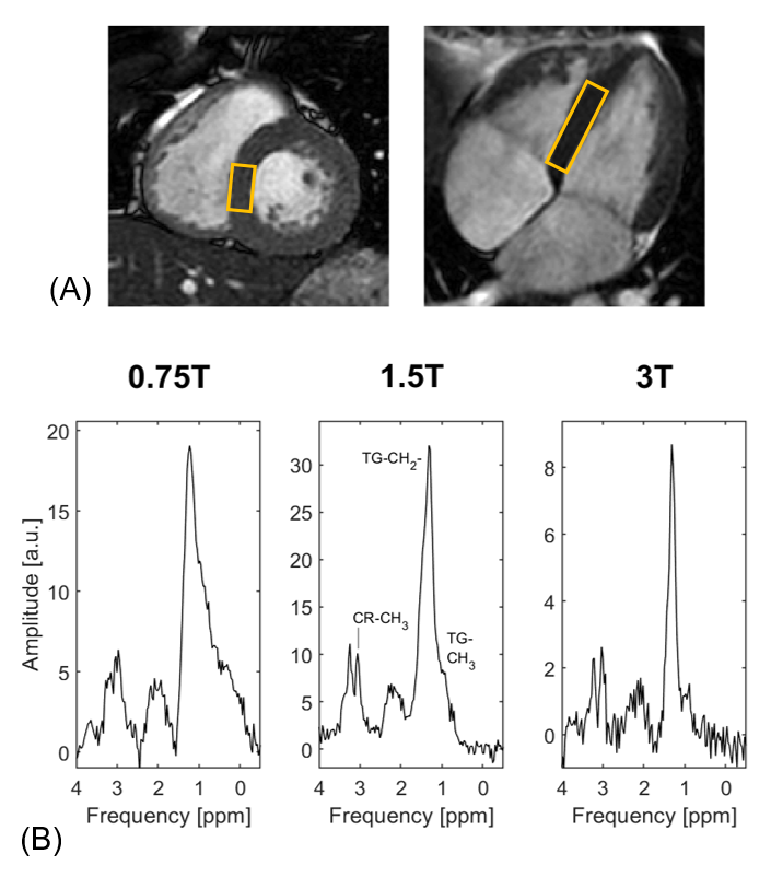
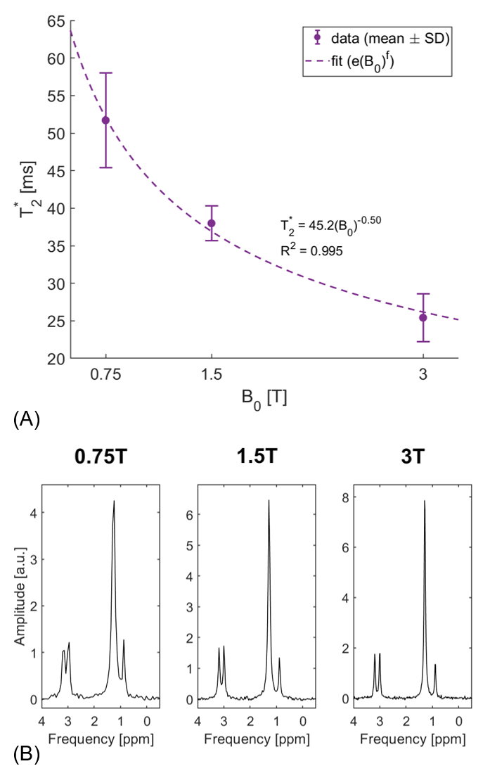
Exemplary spectra acquired from the soleus muscle from one volunteer at 0.75T, 1.5T and 3T are shown in Figure 2. Both triglycerides and creatine can be clearly distinguished in all three spectra. In Figure 3 the T₁, T₂ and T₂^* dependencies on field strength for the water signal of in vivo calf muscle are presented. T₁ increases with increasing field strength, whereas both T₂ and T₂^* decrease. Figure 4 compares exemplary spectra acquired in the interventricular septum of one subject at different field strengths. Even though peak separation decreases for lower field strengths, both TG and CR can be detected at 0.75T. Figure 5 shows T₂^* of myocardial water fitted as a function of magnetic field strength. This corresponds with linewidths of 6.22±0.74 Hz (0.75T), 8.40±0.51 Hz (1.5T) and 12.65±1.57 Hz (3T). Simulated spectra for different field strengths based on these T₂^* values, physiological metabolite relaxation parameters and realistic SNR values show that creatine can still be distinguished from TMA at 0.75T.

Discussion

Although peak separation is reduced at low field, prolonged T₂^* makes spectral quality adequate to distinguish relevant metabolites. Decreased T₁ values, increased T₂ values, decreased echo times and the possibility to decrease receiver bandwidth can all lead to an increase in signal and are therefore clear advantages of lower fields. Chemical shift artefacts increase as a function of magnetic field strength, leading to better spatial localization at lower field strengths.
The absence of a body coil for RF transmission at 0.75T was a limitation in this study; B₁ power optimization was therefore challenging and the B₁⁺ field was inhomogeneous. Local power optimization could, however, be performed for the spectroscopic measurements.

Conclusion

Both measurements and simulations using first principles indicate that human in vivo proton spectroscopy in skeletal muscle and in the heart is achievable at 0.75T.

Acknowledgements

No acknowledgement found.