4000
Scan Efficiency Optimisation for Quantitative Susceptibility Mapping of White Matter at 7T.1Centre for the Developing Brain, School of Biomedical Engineering & Imaging Sciences, King’s College London, London, United Kingdom, 2Biomedical Engineering Department, School of Biomedical Engineering & Imaging Sciences, King’s College London, London, United Kingdom, 3MR Research Collaborations, Siemens Healthcare Limited, Frimley, United Kingdom, 4MRI Group, Department of Medical Physics and Biomedical Engineering, University College London, London, United Kingdom
Synopsis
Quantitative Susceptibility Mapping (QSM) used for microstructural assessment of white matter (WM) is very attractive at ultra high magnetic field strengths, due to the increased signal-to-noise ratio (SNR) and phase sensitivity. This allows shortening echo and repetition times and, therefore, acquisition time. Further advantages of QSM are the low flip angles used for scanning, which results in low specific absorption rates, and the B1 insensitivity of the signal phase. However, suboptimal choice of imaging parameters will result in suboptimal SNR. The purpose of this work is to find and test optimal scanning parameters for QSM of the WM at 7T.
INTRODUCTION
Quantitative Susceptibility Mapping (QSM) used for microstructural assessment of white matter (WM)1 is very attractive at ultra high magnetic field (UHF) strengths, due to the increased signal-to-noise ratio (SNR) and phase sensitivity. This allows shortening echo and repetition times and, therefore, acquisition time. Further advantages of QSM are the low flip angles used for scanning, which results in low specific absorption rates (SAR), and the B1 insensitivity of the signal phase.2,3 However, suboptimal choice of imaging parameters will result in suboptimal SNR. The purpose of this work is to find and test optimal scanning parameters for QSM of the WM at 7T.METHODS
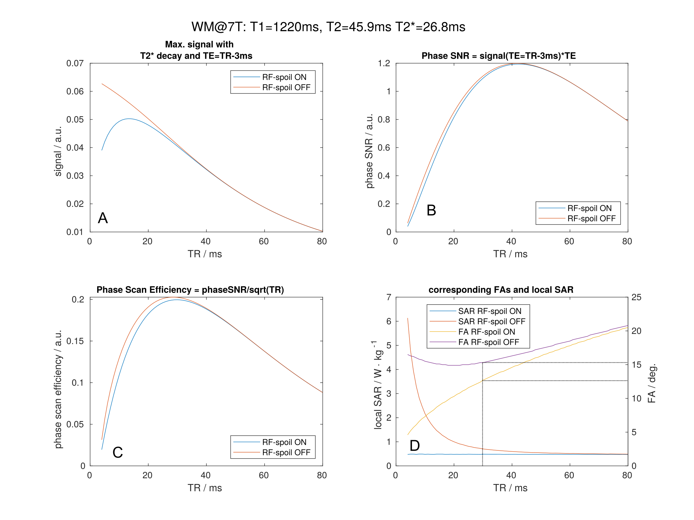
The gradient echo (GRE) signal in the WM was calculated using the equations for RF spoiled4 and unspoiled5 GRE:$$S_{RFspoilON}=\frac{\sin\!FA\,(1-e^{-TR\diagup T_1})}{(1-\cos\!FA\,e^{-TR\diagup\,T_1})}e^{-TE\diagup\,T_2^*}\qquad\qquad\qquad\,\,(1)\\S_{RFspoilOFF}=\tan\!\left(\frac{FA}{2}\right)\left(1-\frac{(E_1-\cos\!FA)(1-E_2^2)}{\sqrt{p^2-q^2}}\right)\qquad(2)\\\text{with}\,E_1=e^{-TR\diagup T_1},\,E_1=e^{-TR\diagup\,T_2}\qquad\qquad\qquad\\p=1-E_1\cos\!FA-E_2^2(E_1-\cos\!FA)\\q=E_2(1-E_1)(1+\cos\!FA)\qquad\quad\,\,\\\text{and the WM relaxation times at 7T:}\qquad\qquad\qquad\\T_1=1220\text{ms},^6\,T_2=45.9\text{ms},^7\,\text{and}\,T_2^*=26.8\text{ms}.^8$$
The echo time (TE) was set to be 3ms shorter than the repetition time (TR) to accommodate rephase and spoiler gradients after the readout. The resulting maximum WM signals from Equation 1 and 2 for a given TR and its corresponding FA are shown in Fig.1. The phase SNR was calculated by multiplying the phase sensitivity, which increases linearly with TE, with the maximum WM signal for a given TR. The WM scanning efficiency of the GRE phase images was then calculated by dividing the phase SNR by the square root of the TR.
A healthy volunteer (male, 29y) was scanned on a MAGNETOM Terra (Siemens Healthcare, Erlangen, Germany) 7T MRI scanner in clinical mode using the 1/32 transmit/receive head coil (Nova Medical, Wilmington MA, USA) with informed consent and Institutional Research Ethics Committee approval. Multi echo GRE images for QSM were acquired with the following parameters: TEs=2.68/7.37/12.06/16.75/21.44/26.13ms, TR=29ms, RF spoil ON with FAs=12.5 and 15.5° and RF spoil OFF with FAs=15.5 and 19° (see results and below for further information), isotropic 0.7mm voxel size and 2x2 parallel acquisition acceleration using CAIPIRINHA9 and scan time for each acquisition 5:35min.
To better assess the effect of the RF spoiling on the signal, the scan with RF spoiling ON was repeated with FA=15.5° to match the optimal FA of the scan with RF spoiling OFF. The impact on the signal of such a 24% FA increase was also tested for the scan with RF spoil OFF, which was repeated with 19° FA.
The data sets were realigned to the mean of all scans using FSL-FLIRT10 the realignment was repeated twice with an updated reference. The brain was extracted using FSL BET.11
All processing used MATLAB (The Mathworks Inc., Natick MA, USA). R2* maps were computed using the Moore-Penrose pseudoinverse. For QSM, the phase images of each receive channel were combined using the phase difference between two consecutive echoes, which eliminates the individual coil sensitivities. Complex fitting12 was used to fit the phase over all TEs and the local phase was extracted by Laplacian background field removal.13 Susceptibility calculation used Iterative Tikhonov regularisation (α=0.05).14
RESULTS
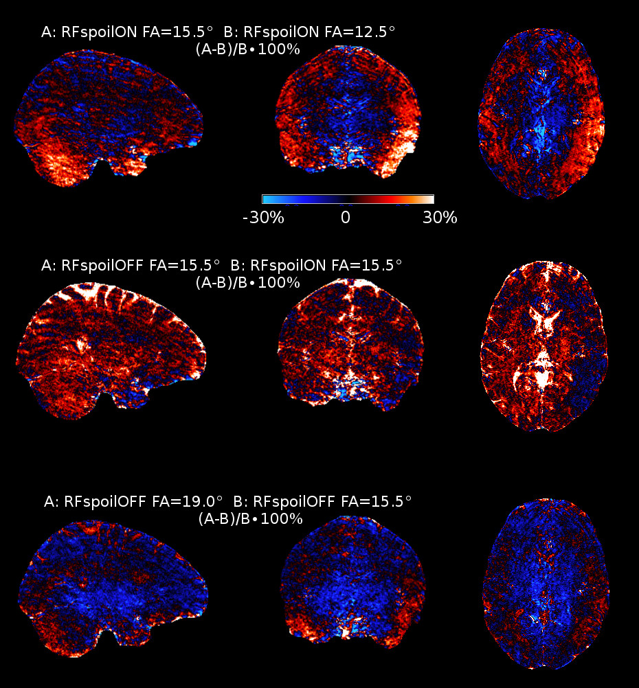
Figure 1A shows that the maximum WM signal declines with increasing TR with RF spoiling OFF, while with RF spoiling ON the signal is also low for shorter TRs. However, the phase SNR for short TRs does not greatly differ between RF spoiling ON or OFF, because it is already low due to the even shorter TEs (Fig.1B). Consequently, the efficiency for scanning the WM phase shows no substantial difference between RF spoiling ON or OFF (Fig.1C). In both cases the most efficient TR is 29ms. The corresponding FAs shown in Fig.1D are rounded to the closest 0.5° FA increment of the scanner with FA=12.5° for RF spoiling ON and FA=15.5° for RF spoiling OFF.Signal difference maps between the scans with different FAs, but RF spoil ON, (Fig.2,top) show up to 30% signal increase for cerebellar and temporal regions. These regions typically suffer from low B1 with similar (single transmit, multi receive) head coils at 7T. The centre of the brain, which has higher B1 in this setting, shows signal loss due to increased saturation caused by the increased FA. The comparison between the two scans with RF spoiling ON/OFF, but equal FAs, shows an overall signal gain which is very strong for CSF (Fig.2,middle). CSF benefits especially from switching RF spoiling OFF, due to its long T2.15 Increasing the FA for RF spoiling OFF shows overall more signal losses than gains (Fig.2,bottom).
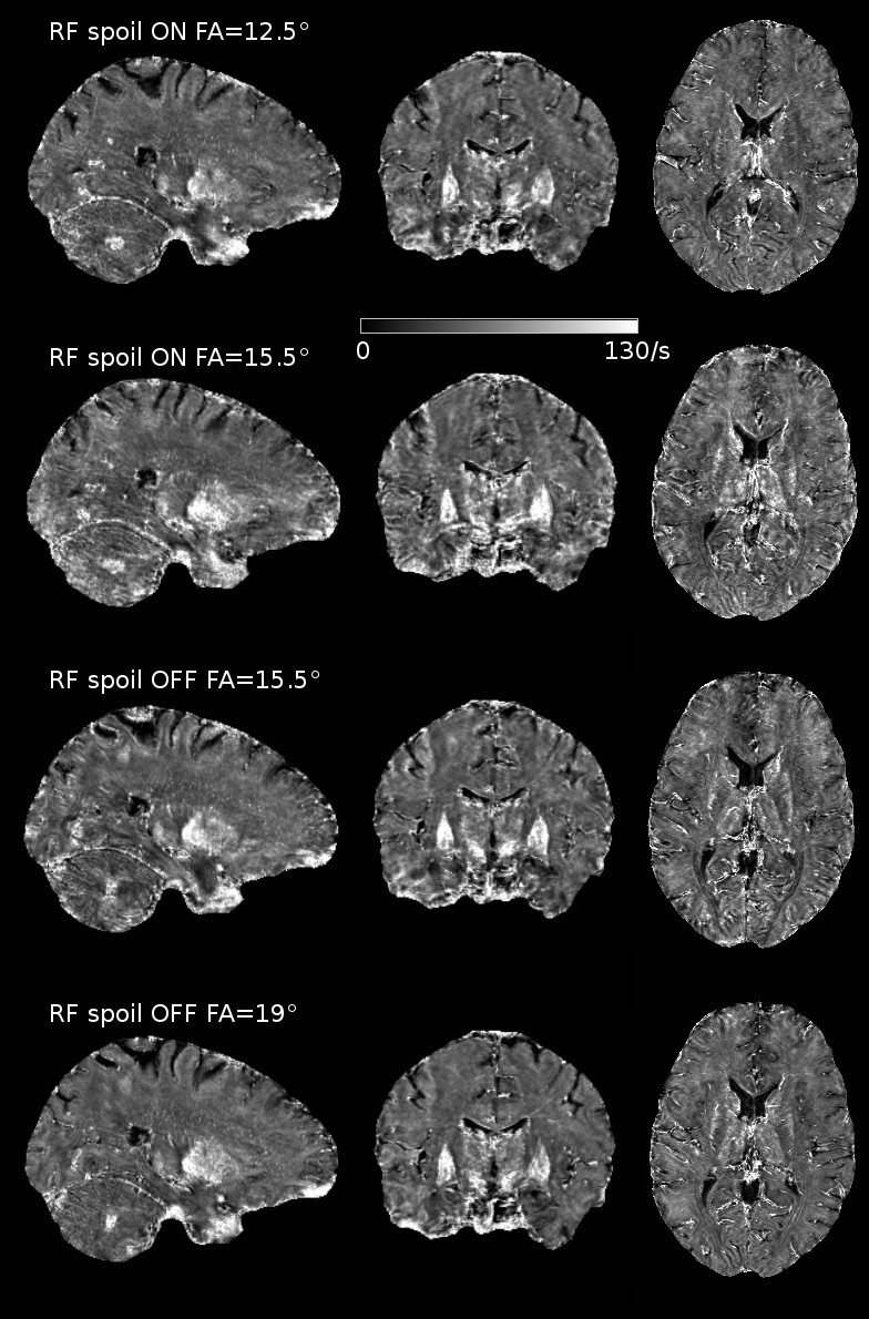
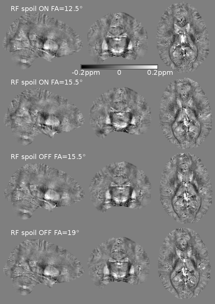
R2* maps show some visual differences most likely caused by subject motion during data acquisition (Fig.3). The QSM maps appear even more similar between the different scanning options (Fig.4).
DISCUSSION & CONCLUSION
QSM at 7T for assessing WM microstructure has maximum scan efficiency using RF spoiling OFF, TR=29ms and FA=15.5°. Increasing the flip angle to compensate for low B1 regions did not improve the overall signal magnitude of these optimal scan parameters. The different scan options do not obviously impact the R2* and QSM maps. However, a further quantitative analysis of these maps and more scanned subjects may show subtle differences. Based on the demonstrated signal increase it is advantageous to acquire QSM using the found optimal scanning parameters.Acknowledgements
This work was supported by Wellcome Trust Collaboration in Science Award 201526/Z/16/Z, the Wellcome EPSRC Centre for Medical Engineering at Kings College London (WT 203148/Z/16/Z) and by the National Institute for Health Research (NIHR) Biomedical Research Centre based at Guy’s and St Thomas’ NHS Foundation Trust and King’s College London. The views expressed are those of the authors and not necessarily those of the NHS, the NIHR or the Department of Health.References
1. Marques JP, Khabipova D, Gruetter R. Studying cyto and myeloarchitecture of the human cortex at ultra-high field with quantitative imaging: R1, R2* and magnetic susceptibility. Neuroimage. 2017 Feb 15;147:152-163.
2. Abduljalil AM, Schmalbrock P, Novak V, Chakeres DW. Enhanced gray and white matter contrast of phase susceptibility-weighted images in ultra-high-field magnetic resonance imaging. J Magn Reson Imaging. 2003 Sep;18(3):284-90.
3. Deistung A, Rauscher A, Sedlacik J, Stadler J, Witoszynskyj S, Reichenbach JR. Susceptibility weighted imaging at ultra high magnetic field strengths: theoretical considerations and experimental results. Magn Reson Med. 2008 Nov;60(5):1155-68.
4. Ernst, R. R., and W. A. Anderson. 1966. “Application of Fourier Transform Spectroscopy to Magnetic Resonance.” Review of Scientific Instruments 37 (1): 93–102.
5. Hänicke, Wolfgang, and Horst U. Vogel. 2003. “An Analytical Solution for the SSFP Signal in MRI.” Magnetic Resonance in Medicine 49 (4): 771–75.
6. Rooney, William D., Glyn Johnson, Xin Li, Eric R. Cohen, Seong-Gi Kim, Kamil Ugurbil, and Charles S. Springer. 2007. “Magnetic Field and Tissue Dependencies of Human Brain Longitudinal 1H2O Relaxation in Vivo.” Magnetic Resonance in Medicine 57 (2): 308–18.
7. Yacoub, Essa, Timothy Q. Duong, Pierre-Francois Van De Moortele, Martin Lindquist, Gregor Adriany, Seong-Gi Kim, Kâmil Uğurbil, and Xiaoping Hu. 2003. “Spin-Echo FMRI in Humans Using High Spatial Resolutions and High Magnetic Fields.” Magnetic Resonance in Medicine 49 (4): 655–64.
8. Peters, Andrew M., Matthew J. Brookes, Frank G. Hoogenraad, Penny A. Gowland, Susan T. Francis, Peter G. Morris, and Richard Bowtell. 2007. “T2* Measurements in Human Brain at 1.5, 3 and 7 T.” Magnetic Resonance Imaging 25 (6): 748–53.
9. Breuer FA, Blaimer M, Mueller MF, et al. 2006. “Controlled aliasing in volumetric parallel imaging (2D-CAIPIRINHA).” Magnetic Resonance in Medicine 55: 549–556.
10. M. Jenkinson and S.M. Smith. A global optimisation method for robust affine registration of brain images. Medical Image Analysis, 5(2):143-156, 2001.
11. S.M. Smith. Fast robust automated brain extraction. Human Brain Mapping, 17(3):143-155, November 2002.
12. Liu T, Wisnieff C, Lou M, Chen W, Spincemaille P, Wang Y. Nonlinear formulation of the magnetic field to source relationship for robust quantitative susceptibility mapping. Magn Reson Med. 2013 Feb;69(2):467-76.
13. Schweser F, Deistung A, Lehr BW, Reichenbach JR. Quantitative imaging of intrinsic magnetic tissue properties using MRI signal phase: an approach to in vivo brain iron metabolism? Neuroimage. 2011 Feb 14;54(4):2789-807.
14. Karsa, A, Punwani, S, Shmueli, K, et al. An optimized and highly repeatable MRI acquisition and processing pipeline for quantitative susceptibility mapping in the head‐and‐neck region. Magn Reson Med. 2020; 84: 3206– 3222.
15. Daoust, A., S. Dodd, G. Nair, N. Bouraoud, S. Jacobson, S. Walbridge, D. S. Reich, and A. Koretsky. 2017. “Transverse Relaxation of Cerebrospinal Fluid Depends on Glucose Concentration.” Magnetic Resonance Imaging 44: 72–81.
Figures