3983
Improving Quantitative Susceptibility Mapping reconstructions via non-linear Huber loss data fidelity term (Huber-QSM)1Department of Electrical Engineering, Pontificia Universidad Católica de Chile, Santiago, Chile, 2Biomedical Imaging Center, Pontificia Universidad Católica de Chile, Santiago, Chile, 3Millennium Nucleus for Cardiovascular Magnetic Resonance, Santiago, Chile, 4Department of Medical Physics and Biomedical Engineering, University College London, London, United Kingdom
Synopsis
Compared to L2-norm based QSM reconstructions, methods based on L1-norm data consistency are less prone to artifact generation caused by phase inconsistencies (e.g. unwrapping artifacts, intravoxel dephasing). However, L2-norm methods present better denoising performance in high SNR regions. Here, we present a QSM algorithm that combines the strengths of the L1 and L2 norms, using Huber's loss function as the data consistency term. Simulations and in vivo reconstructions showed enhanced performance, with superior artifact suppression capabilities of our proposed method.
Introduction
Susceptibility maps are estimated by solving an ill-posed inverse problem. The source-to-field problem is modeled by a magnetic dipole convolution. The magnetic dipole kernel has a zero-valued biconical surface in the frequency space1,2. This singularity makes the noise propagate through the reconstructed maps generating the so-called streaking artifacts3. QSM reconstruction algorithms with data consistencies based the L1-norm probed to be more robust against phase outliers than those using the L2-norm, preventing the generation of artifacts4. However, L2-norm based methods have shown better noise management on high SNR regions. In this paper we present a new data consistency term that combines the L1 and L2 norms by using the Huber loss5.Methods
The proposed method consists in solving the following nonlinear functional6,7:$$\underset{\chi}{\text{argmin }}h_{\delta}\left(w\left(e^{iF^{H}DF\chi}-e^{i\phi}\right)\right)+\lambda\cdot TV\left(\chi\right)$$
where $$$F$$$ is the Fourier transform with its inverse $$$F^H$$$, $$$D$$$ is the dipole kernel, $$$\phi$$$ is the tissue phase, $$$\chi$$$ is the susceptibility distribution, $$$w$$$ is a magnitude-based weight or ROI binary mask, $$$TV\left(x\right)$$$ is the total variation regularizer8, and $$$\lambda$$$ is the regularization weight. $$$h_{\delta}\left(x\right)$$$ is the Huber loss defined by:
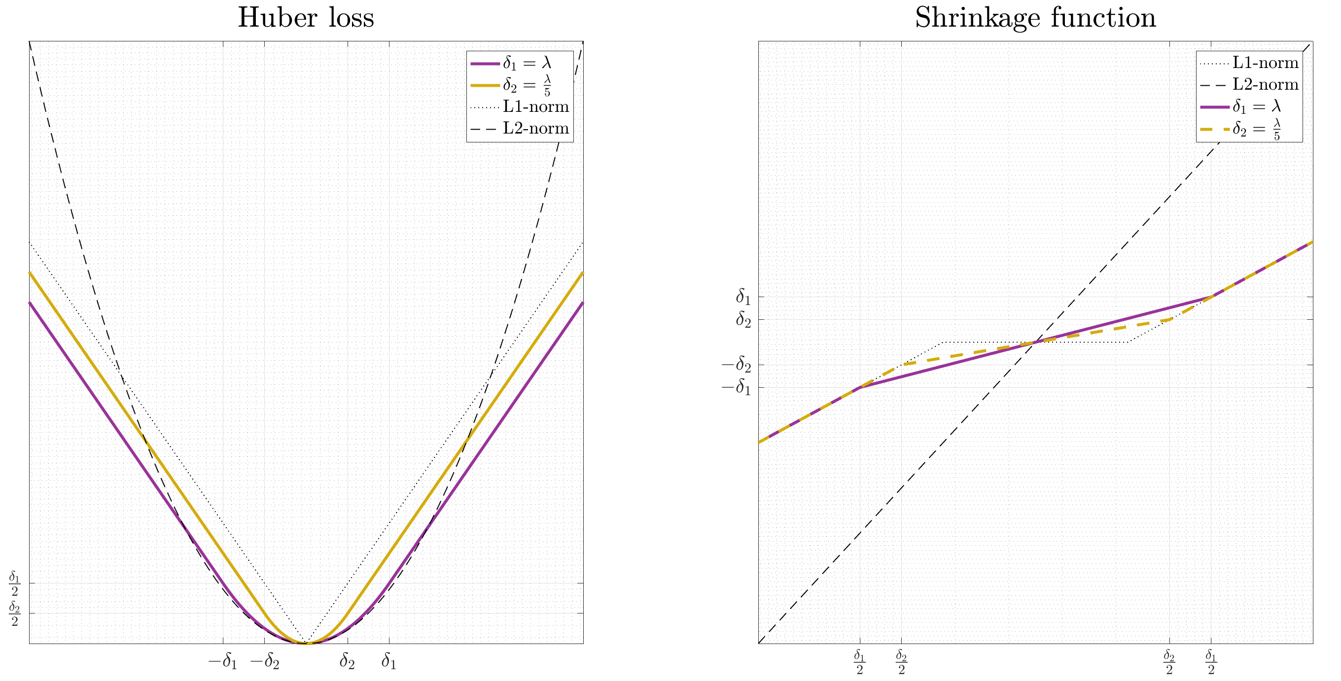
$$h_{\delta}\left(x\right)=\begin{cases} \frac{1}{2\cdot\delta}x^{2} & \left|x\right|\leq\delta\\ \left|x\right|-\frac{\delta}{2} & \left|x\right|>\delta \end{cases}$$
where $$$\delta > 0$$$ is the threshold parameter. We solve this optimization problem using the ADMM framework9. To decouple the data fidelity term, we add the following auxiliary variables $$$z_1=F^{H}DF\chi$$$ and $$$z_2=e^{iz_1}-e^{i\phi}$$$. The $$$z_1$$$ subproblem is solved as shown earlier for the L1-norm4,7, with a Newton-Raphson iterative approach. The solution of the $$$z_2$$$ subproblem is given by the following shrinkage function:
$$z_{2}=\frac{\delta\cdot\mu_{2}\cdot\left(e^{iz_{1}}-e^{i\phi}+s_{2}\right)+w^{2}\cdot\max\left(\left|e^{iz_{1}}-e^{i\phi}+s_{2}\right|-\frac{w^{2}+\mu_{2}\cdot\delta}{w\cdot\mu_{2}},\;0\right)\cdot\text{sign}\left(e^{iz_{1}}-e^{i\phi}+s_{2}\right)}{w^{2}+\delta\cdot\mu_{2}}$$
Figure 1 shows the cost and shrinkage functions of $$$h_{\delta}\left(x\right)$$$, L1-norm and L2-norm.
We compared the proposed method (nlHu) with non-linear L2-norm (FANSI)7 and non-linear L1-norm (nlL1)4 methods, all with total variation regularization, in the following experiments:
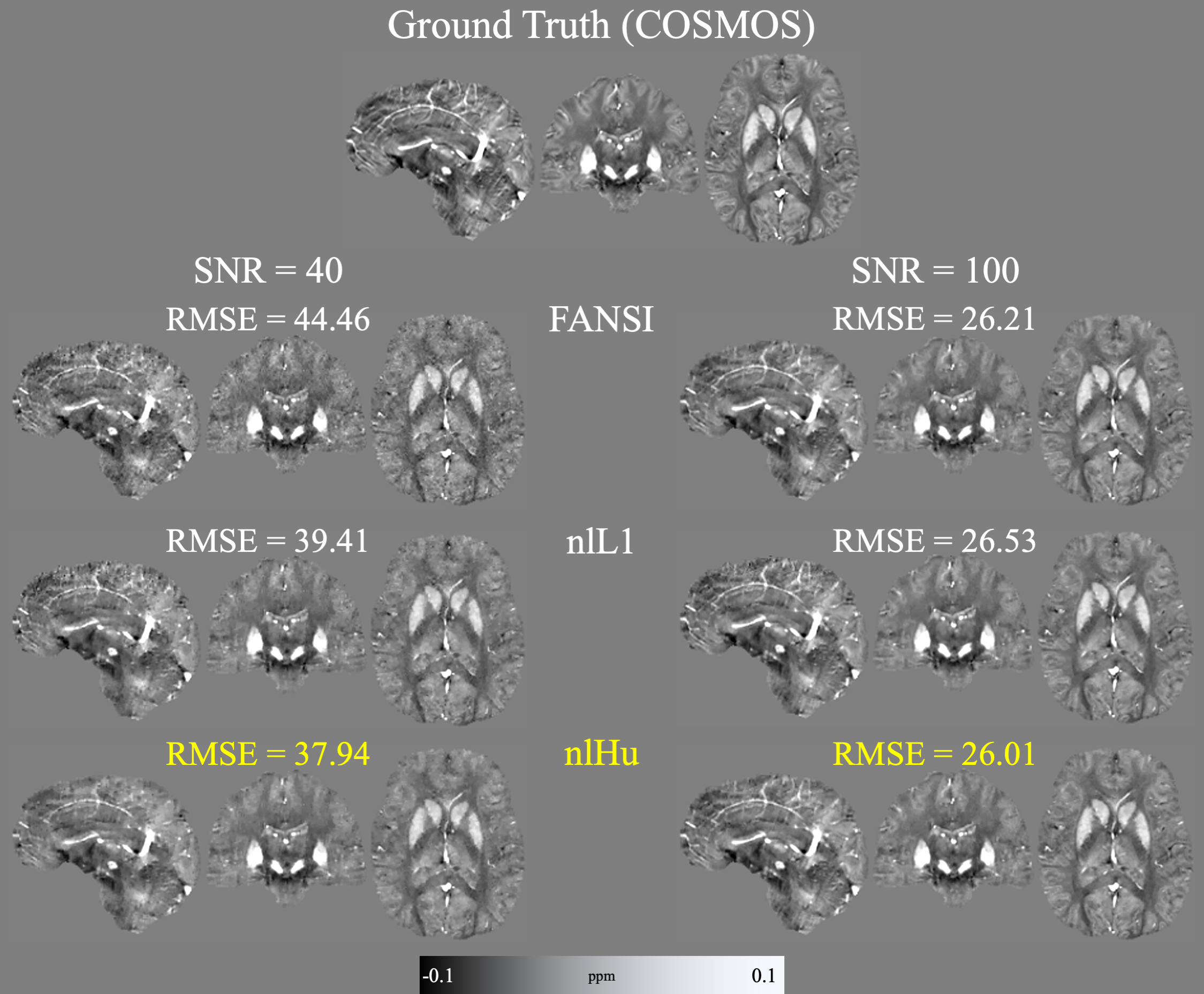
- COSMOS forward simulations: From a COSMOS10 brain reconstruction (2016 QSM challenge dataset11) we synthetized the local phase and added complex noise to the complex image (SNR=40 and SNR=100). In addition, two simulated lesions were added, one paramagnetic (-0.5 ppm) and one diamagnetic (0.2 ppm), to mimic highly noisy phase inconsistencies.
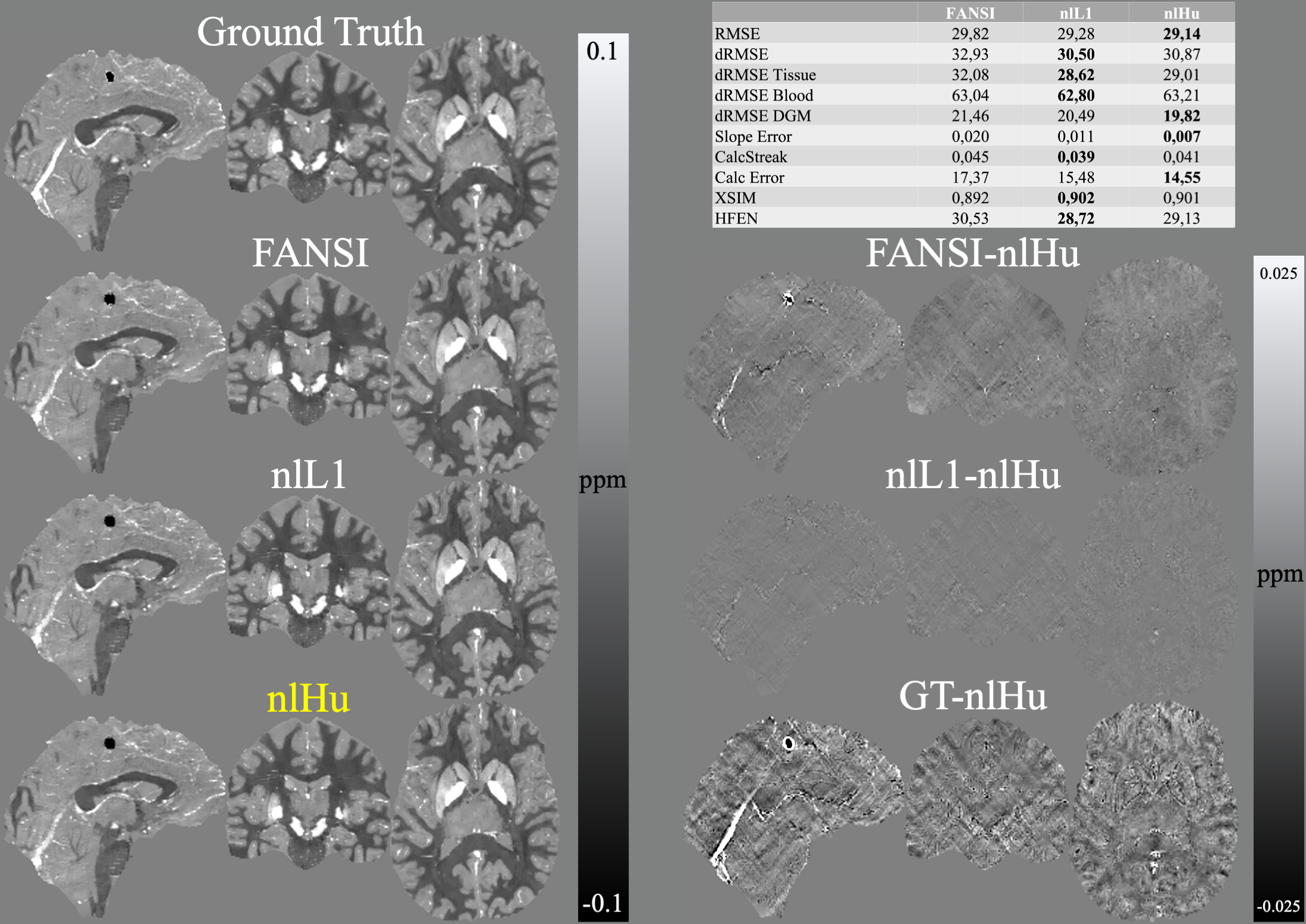
- SIM2SNR1: Using the SIM2SNR1 dataset (2019 QSM challenge)12,13 we compared the performance using the official metrics, plus HFEN14 and XSIM15. We used multi-echo data and masked magnitude-based weight. For the inversions we used a zero-padding to form a volume of 256x256x256 voxels.
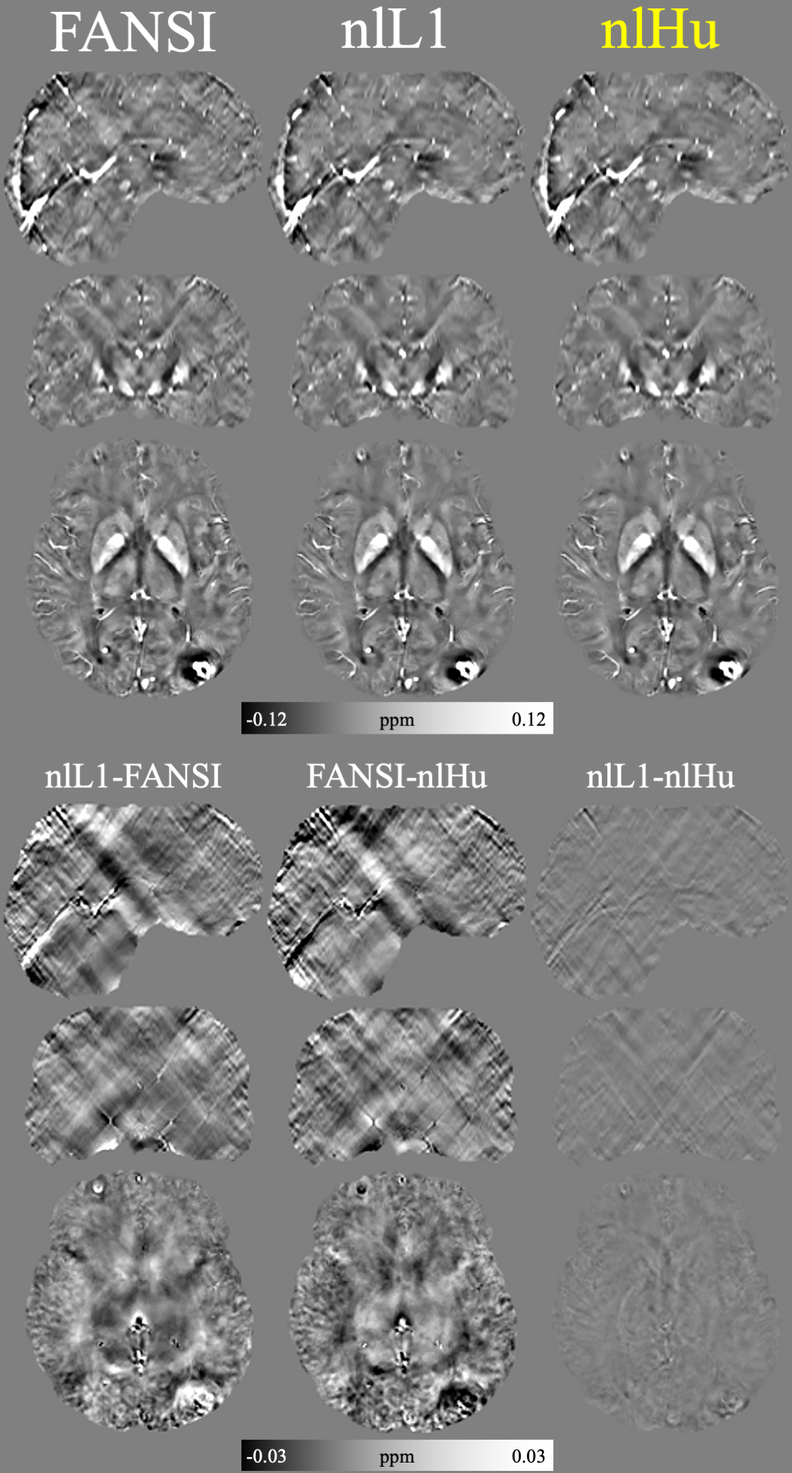
- IN-VIVO Data: Siemens 3T scanner (Magnetom Trio Tim; Siemens Healthcare, Erlangen, Germany) with a 12-channel phased-array head coil. GRE sequence with 6 echoes. A patient showing extensive bleeding was scanned with the following sequence parameters: TE1=4.92ms, ΔTE=4.92ms, TR=35ms, flip angle=15°, 232×288×64 matrix with 0.8×0.8×2mm3 voxels, and Tacq=4:51min. 1. We performed Laplacian phase unwrapping16 and background field removal using PDF17 and VSHARP18.
Results
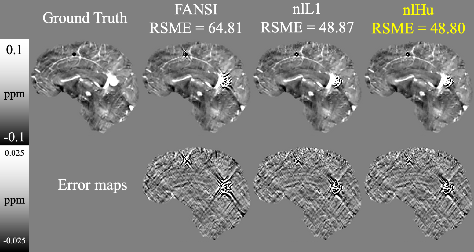
Figure 2 presents the COSMOS-based reconstructions for both SNR levels, at both noise levels nlHu obtained the lowest RMSE. Figure 3 presents the sagittal slices of reconstructions of SNR=100 with the simulated lesions. SIM2SNR1 reconstructions are presented in Figure 4, along with difference maps and a table with the performance metrics. In-vivo reconstructions and difference maps are shown in Figure 5.Discussion & Conclusion
In Figure 2, we can see that in comparison to FANSI, nlHu manages to reconstruct the veins in the cortical zone more effectively. In the same figure we can see that nL1 reconstructions have a noisier appearance than nlHu. In Figure 3 we can see that nlHu manages to stop the propagation of streaking artifacts. The metrics obtained in experiment 2 show that nlHu has better performance than FANSI and similar performance to nlL1. However, the results of the other experiments show that nlHu has a better performance than nlL1 in areas with high SNR. Although nlHu has one additional parameter over FANSI, optimizing it does not require much effort. Our simulated experiments revealed a convex behavior of $$$\delta$$$ on the RMSE, whereas it is possible to fine-tune the regularization parameter ($$$\lambda$$$) first and then $$$\delta$$$. The experiments we conducted show the importance of the term data consistency in noise reduction. The Huber loss combines the strengths of the L1 and L2 norms into a single term.Acknowledgements
This work has been funded by projects Fondecyt 1191710, PIA-ACT192064, and the Millennium Nucleus on Cardiovascular Magnetic Resonance of the Millennium Science Initiative NCN17_129, by the National Agency for Research and Development, ANID.
We thank Dr. Christian Langkammer from the Medical University of Graz, Austria, for sharing his data with us and for his support.
References
- Salomir, R., De Senneville, B. D., & Moonen, C. T. W. (2003). A fast calculation method for magnetic field inhomogeneity due to an arbitrary distribution of bulk susceptibility. Concepts in Magnetic Resonance Part B: Magnetic Resonance Engineering, 19(1), 26–34. https://doi.org/10.1002/cmr.b.100832.
- Marques, J. P., & Bowtell, R. (2005). Application of a fourier-based method for rapid calculation of field inhomogeneity due to spatial variation of magnetic susceptibility. Concepts in Magnetic Resonance Part B: Magnetic Resonance Engineering, 25(1), 65–78. https://doi.org/10.1002/cmr.b.200343.
- Shmueli, K., De Zwart, J. A., Van Gelderen, P., Li, T. Q., Dodd, S. J., & Duyn, J. H. (2009). Magnetic susceptibility mapping of brain tissue in vivo using MRI phase data. Magnetic Resonance in Medicine, 62(6), 1510–1522. https://doi.org/10.1002/mrm.221354.
- Milovic C, Lambert M, Langkammer C, Bredies K, Tejos C, Irarrazaval P. QSM streaking suppression with L1 data fidelity terms . In: Proc. Intl. Soc. Mag. Reson. Med. 2020;p3257.5.
- Huber, P. J. (1964). Robust Estimation of a Location Parameter. The Annals of Mathematical Statistics, 35(1), 73-101.
- Liu T, Wisnieff C, Lou M, Chen W, Spincemaille P, Wang Y. Nonlinear formulation of the magnetic field to source relationship for robust quantitative susceptibility mapping. Magn Reson Med 2013;69:467–476.
- Milovic, Carlos, Bilgic, Berkin, Zhao, Bo, Acosta-Cabronero, Julio, & Tejos, Cristian. (2018). Fast nonlinear susceptibility inversion with variational regularization. Magnetic Resonance in Medicine, 80(2), 814-821.
- Dai-Qiang Chen, & Li-Zhi Cheng. (2012). Spatially Adapted Total Variation Model to Remove Multiplicative Noise. IEEE Transactions on Image Processing, 21(4), 1650-1662. 9.
- Bilgic, B., Chatnuntawech, I., Langkammer, C., & Setsompop, K. (2015). Sparse methods for Quantitative Susceptibility Mapping. Wavelets and Sparsity XVI, 9597, 959711. https://doi.org/10.1117/12.2188535
- Liu T, Spincemaille P, De Rochefort L, Kressler B, Wang Y. Calculation of susceptibility through multiple orientation sampling (COSMOS): a method for conditioning the inverse problem from measured magnetic field map to susceptibility source image in MRI. Magn Reson Med 2009;61:196–204.
- Langkammer C, Schweser F, Shmueli K, et al. Quantitative susceptibility mapping: report from the 2016 reconstruction challenge. Magn Reson Med 2018;79:1661–1673.
- Bilgic, B., Langkammer, C., Marques, J. P., Meineke, J., Milovic, C., & Schweser, F. (pre-print). QSM Reconstruction Challenge 2.0: Design and Report of Results. BioRxiv.
- Marques et al. Part 1. BioRxiv.
- Saiprasad R, Bresler Y. MR image reconstruction from highly undersampled k-space data by dictionary learning. IEEE Trans Med Imag- ing 2011;30:1028–1041.
- Milovic C, Tejos C, and Irarrazaval P. Structural Similarity Index Metric setup for QSM applications (XSIM). 5th International Workshop on MRI Phase Contrast & Quantitative Susceptibility Mapping, Seoul, Korea, 2019.
- Li W, Wu B, Liu C. Quantitative susceptibility mapping of human brain reflects spatial variation in tissue composition. NeuroImage 2011;55:1645–1656.
- Liu T, Khalidov I, de Rochefort L, et al. A novel background field removal method for MRI using projection onto dipole fields (PDF). NMR Biomed. 2011;24:1129–1136.
- Li W, Wu B, Liu C. Quantitative susceptibility mapping of human brain reflects spatial variation in tissue composition. NeuroImage 2011;55:1645–1656.
Figures