Introduction

Quantitative susceptibility mapping (QSM) is a MRI technique that estimates tissue magnetic susceptibility. The generation of QSM requires solving a challenging ill-posed field-to-source inversion problem. Recently, several deep learning (DL) QSM techniques[1,2,3,4] have been proposed and demonstrated impressive performance. Due to the inherent non-existent ground-truth QSM references, these techniques used either COSMOS [5] maps or synthetic data for network training. Synthetic data is easy to generate but often adapt poorly to domain shifts. Here, we introduce an easy domain adaption technique using domain-specific batch normalization[6] to improve the domain adaption.

Method

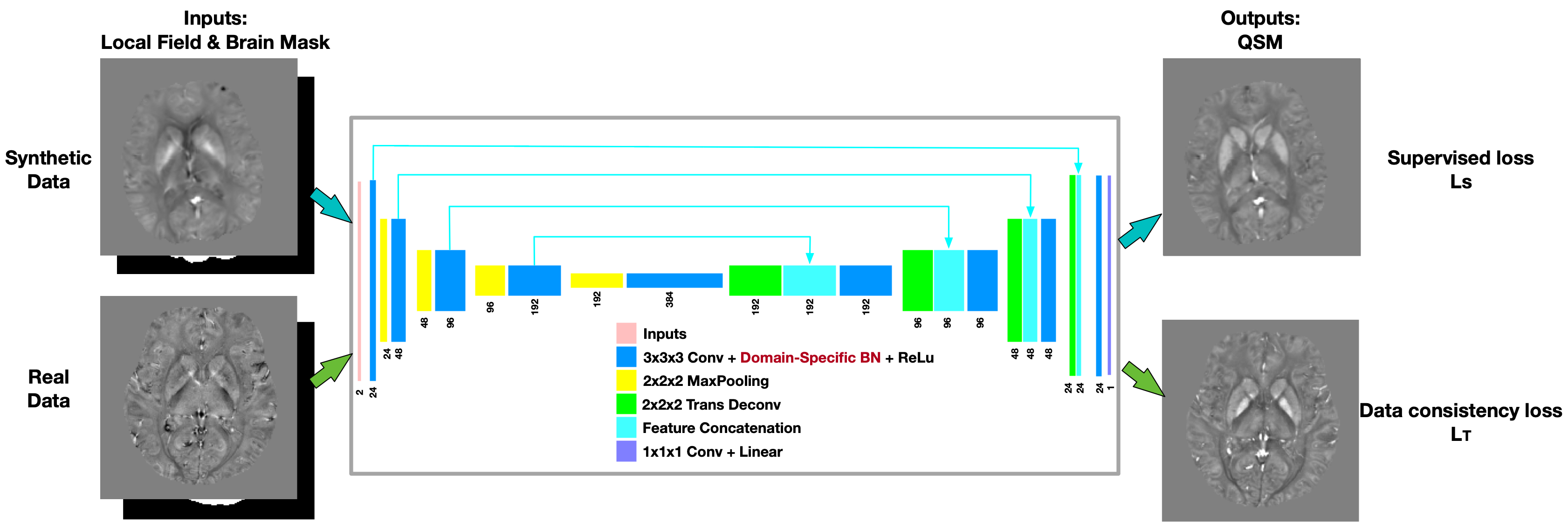
[Neural Network] A modified U-net for 3D data processing was utilized for the dipole inversion, with inputs of local field and brain mask and output of QSM. For the training of the network, whole simulated QSM maps were generated using single brain COSMOS map from 2016 QSM reconstruction challenge and data augmentation techniques (elastic transform, contrast change, and adding lesions). The local field were computed using the dipole kernel convolution. We apply domain-specific batch normalization layers in networks while allowing them to share all other model parameters. For synthetic data, L2 loss was used $$$L_{S} = \left \| \chi _{s} - \chi _{ground truth} \right \|^{2}$$$, where $$$\chi _{s}$$$ is the network QSM output of synthetic data, and $$$\chi _{ground truth}$$$ is the QSM label of synthetic data. For real data, data consistency loss was used $$$L_{T} = \left \| W_{t} (e^{j d\ast \chi _{t}} - e^{j f_{t}}) \right \|^{2}$$$, where $$$W_{t}$$$ is the data weighting term to incorporate the noise weighting term and brain mask, $$$d$$$ is dipole kernel, $$$\chi _{t}$$$ is the network QSM outputs of real data, $$$f_{t}$$$ is local field of real data. Total loss incorporates these two losses $$$L_{Total} = L_{S} + \lambda L_{T}$$$, where $$$\lambda$$$ is loss weight which increases during training. The proposed method is denoted as QSMInvNet+.

[Data] 9 multi-orientation datasets were acquired with 5 head orientations and a 3D single-echo GRE scan with isotropic voxel size 1.0x1.0x1.0mm³ on 3T MRI scanners [1]. The data processing was the same as [9]. For network training, 500 synthetic data were generated then cropped to image patches with patch size 96x96x96 and training data 3000. During training, the RESHARP local field, magnitude image and brain mask of 36 scans (9*4 tilted head positions) were randomly cropped with patch size 96x96x96. QSMInvNet+ was trained using patch-based network with patch size 96x96x96. Adam was used as optimizer with the learning rate of 10-4. The network was implemented using TensorFlow and was trained on one NVIDIA K80 GPU. TKD[7], MEDI[8], COSMOS were performed to get QSM results of normal head position. In addition, DL-based techniques QSMInvNet (which first trained on synthetic data, then fine-tuned the trained model on real data according to the physical model), QSMInvNet+, and uQSM[9] were performed to compare the QSM results. Quantitative metrics such as NRMSE, HFEN, SSIM were calculated using COSMOS result as a reference.

100 clinical data were acquired using susceptibility-weighted angiography on a 3T MRI scanner (GE Healthcare MR750) with data acquisition parameters: in-plane data matrix 288x224, FOV 22 cm, slice thickness 3 mm, first TE 12.6 ms, echo spacing 4.1 ms, 7 echoes, TR 39.7 ms, pixel bandwidth 244 Hz, and total acquisition time of about 2 minutes. Complex multi-echo images were reconstructed from raw k-space data. The brain masks were obtained using the SPM tool. RESHARP method with spherical mean radius 6mm were used for background field removal. For network training, simulated data were generated with voxel size 0.76x0.76x0.76mm³. The network was trained with patch size 128x128x64. TKD, MEDI, QSMInvNet, and QSMInvNet+ were performed to compare the QSM results.

Result

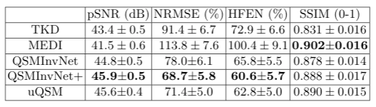
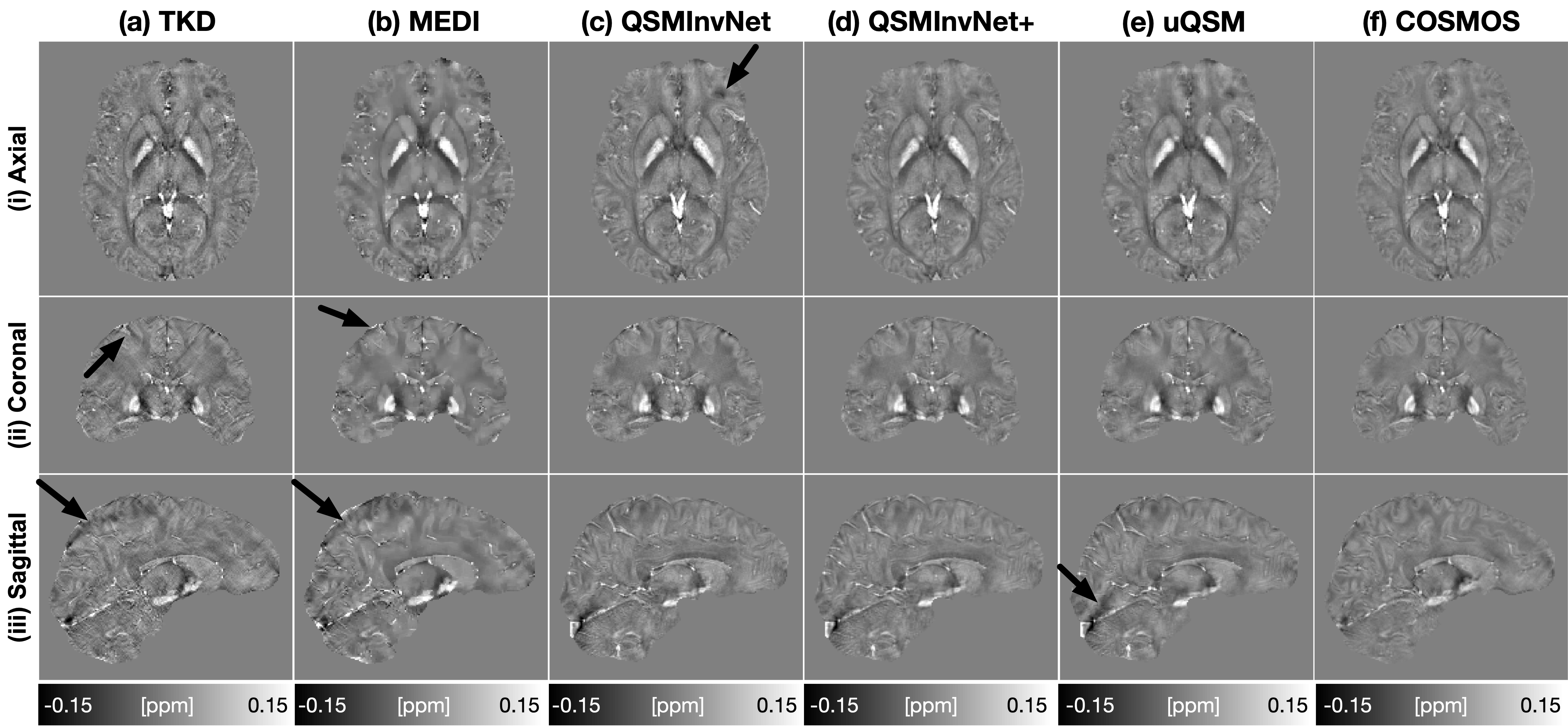
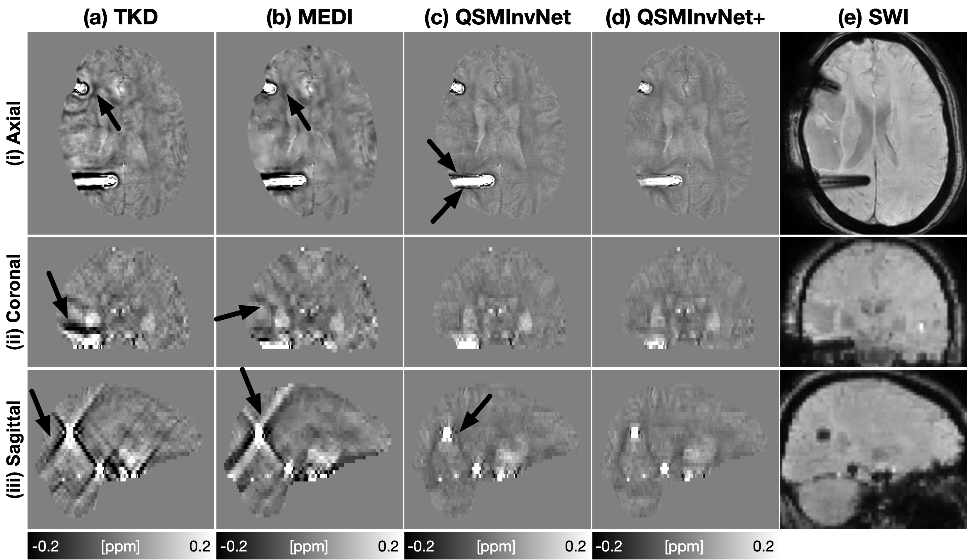
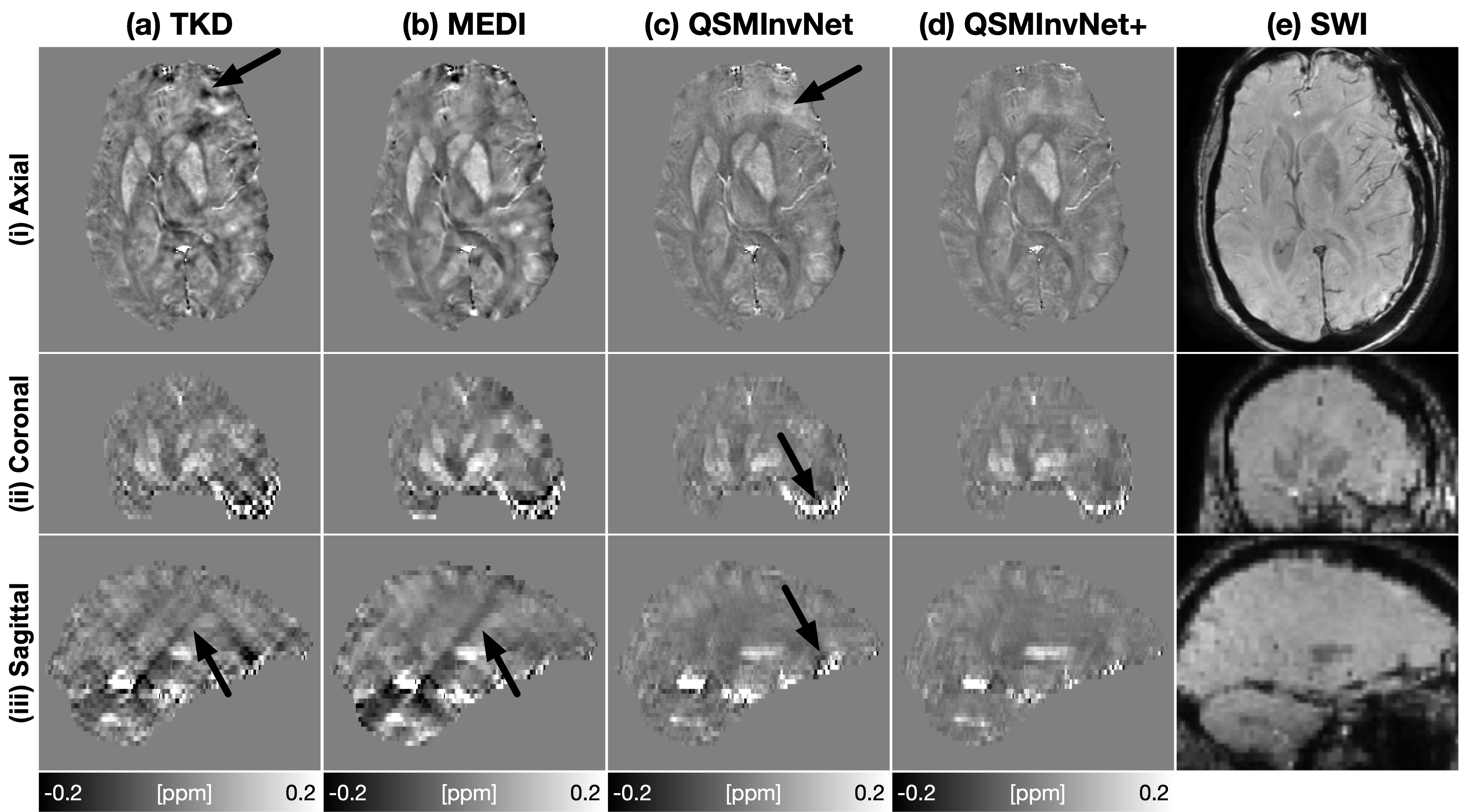
Fig. 2 displays the quantitative metrics of QSM results with COSMOS map as an reference. QSMInvNet+ achieved the best score in PSNR, NRMSE, and HFEN.
Fig. 3 compared QSM results of a multi-orientation dataset. Compared with conventional methods TKD and MEDI, DL-based methods display QSM with clearer details and less artifacts. Among DL-based methods, QSMInvNet+ results shows less shading artifacts. Fig. 4 and Fig. 5 compared QSM results of two clinical datasets with brain hemorrhage. TKD and MEDI results display sever streaking artifact, while QSMInvNet and QSMInvNet+ outperformed with clear details and invisible artifacts. Compared with QSMInvNet, QSMInvNet+ images showed improved performance with less shading artifacts around the lesions.

Discussion and Conclusion

We have proposed to apply domain-specific batch normalization to improve domain adaption of neural networks learning from synthetic data. This method outperforms QSMInvNet - first learning from synthetic data then fine-tuning on real data. Since the method requires simulated data and minor changes on network architecture, it can be easily utilized to facilitate QSM researches.

Acknowledgements

We thank Professor Jongho Lee for sharing the multi-orientation QSM datasets.