3979

Total Deep Variation Regularization for Improved Iterative Quantitative Susceptibility Mapping (TDV-QSM)

Carlos Milovic¹, Jose Manuel Larrain^2,3, and Karin Shmueli¹
¹Department of Medical Physics and Biomedical Engineering, University College London, London, United Kingdom, ²Department of Electrical Engineering, Pontificia Universidad Catolica de Chile, Santiago, Chile, ³Biomedical Imaging Center, Pontificia Universidad Catolica de Chile, Santiago, Chile

Synopsis

Quantitative Susceptibility Mapping (QSM) is an ill-posed inverse problem. Traditionally, it is solved by minimization of a functional. Regularization terms may be interpreted as a denoising process. Many state-of-the-art methods are based on Total Variation regularization terms, with great success. With the advent of Deep Learning, new regularization strategies have been derived from training datasets. Total Deep Variation (TDV) is a recently proposed technique, showing impressive results. We applied a pre-trained TDV network as a denoising step in an iterative QSM solver. Results show improved error metrics for synthetic brain phantoms and enhanced in-vivo reconstructions, compared to Total-Variation-based algorithms.

PURPOSE

Inferring the underlying tissue magnetic susceptibilities from the gradient-echo phase is an ill-posed inverse problem¹, known as Quantitative Susceptibility Mapping (QSM). QSM is typically solved by minimization of a cost functional with a data fidelity term and one or more regularization terms². Whereas the data fidelity term enforces consistency of the solutions with the acquired data and models the noise distribution, regularization terms enforce a-priori knowledge regarding the solution, such as smoothness³ or sparsity. Total Variation (TV)^4,5 and terms derived from it (by introducing local weights4) or extensions such as Total Generalized Variation, TGV^5,6 are popular QSM regularizers, achieving the highest scores in the 2019 QSM Reconstruction Challenge (RC2)⁷. Recent advances in Deep Learning⁸ have provided a new approach to build regularization terms. In particular, variational networks have been successfully applied to denoising and many other linear inverse problems^9,10. Total Deep Variation (TDV)¹¹ is a state-of-the-art variational network, based on the ‘Fields of Experts’ model¹² (a generic framework to learn image priors), but requiring only a fraction of its parameters. This makes TDV easier to train and more generalizable to different problems¹¹. Here, we used a pre-trained (BSDS400 dataset¹³) TDV network (https://github.com/VLOGroup/tdv), designed to remove Gaussian noise from 2D color images, as a proximal (regularization) step within each iteration for QSM reconstruction and evaluated whether it reduced noise and streaking artifacts in the resulting susceptibility maps.

METHODS

In general, we may describe the functional of the QSM inverse problem as $$$argmin_{\chi}F(\chi,\phi)+\alpha R(\chi)$$$, where $$$F(\chi,\phi)$$$ is the data fidelity term between the susceptibility distribution $$$\chi$$$ and the measured phase $$$\phi$$$ (such as the linear³ or nonlinear L2-norm^4,5). $$$R(\chi)$$$ is the regularization term, with $$$\alpha$$$ the Lagrangian weight that balances both terms. To use TDV in an efficient⁵ proximal step, we introduced the $$$z=\chi$$$ variable to split the regularization term from the data fidelity term using the Alternating Directions of Multipliers Method (ADMM) framework^5,14. The augmented functional becomes:
$$argmin_{\chi,z}F(D\chi,\phi)+\alpha R(z)+\frac{\mu}{2}||\chi-z+s||^2_2$$
with $$$\mu$$$ an additional Lagrangian weight, and $$$s$$$ a Lagrange multiplier. Each subproblem is solved consecutively, until convergence. First we solve the $$$\chi$$$ subproblem as previously described in the FANSI⁵ algorithm. Now, the $$$z$$$ subproblem becomes a TDV denoising problem, with input $$$\chi_{k+1}+s_k$$$ at each iteration k, allowing us to use the pre-trained denoising network. The regularization weight $$$\alpha$$$ becomes the scale parameter in TDV that adapts the network to the input noise level. $$$\mu$$$ balances the regularization and the data fidelity terms. Finally, we update $$$s_{k+1}=s_k+\chi_{k+1}-z_{k+1}$$$ and all other Lagrange multipliers.

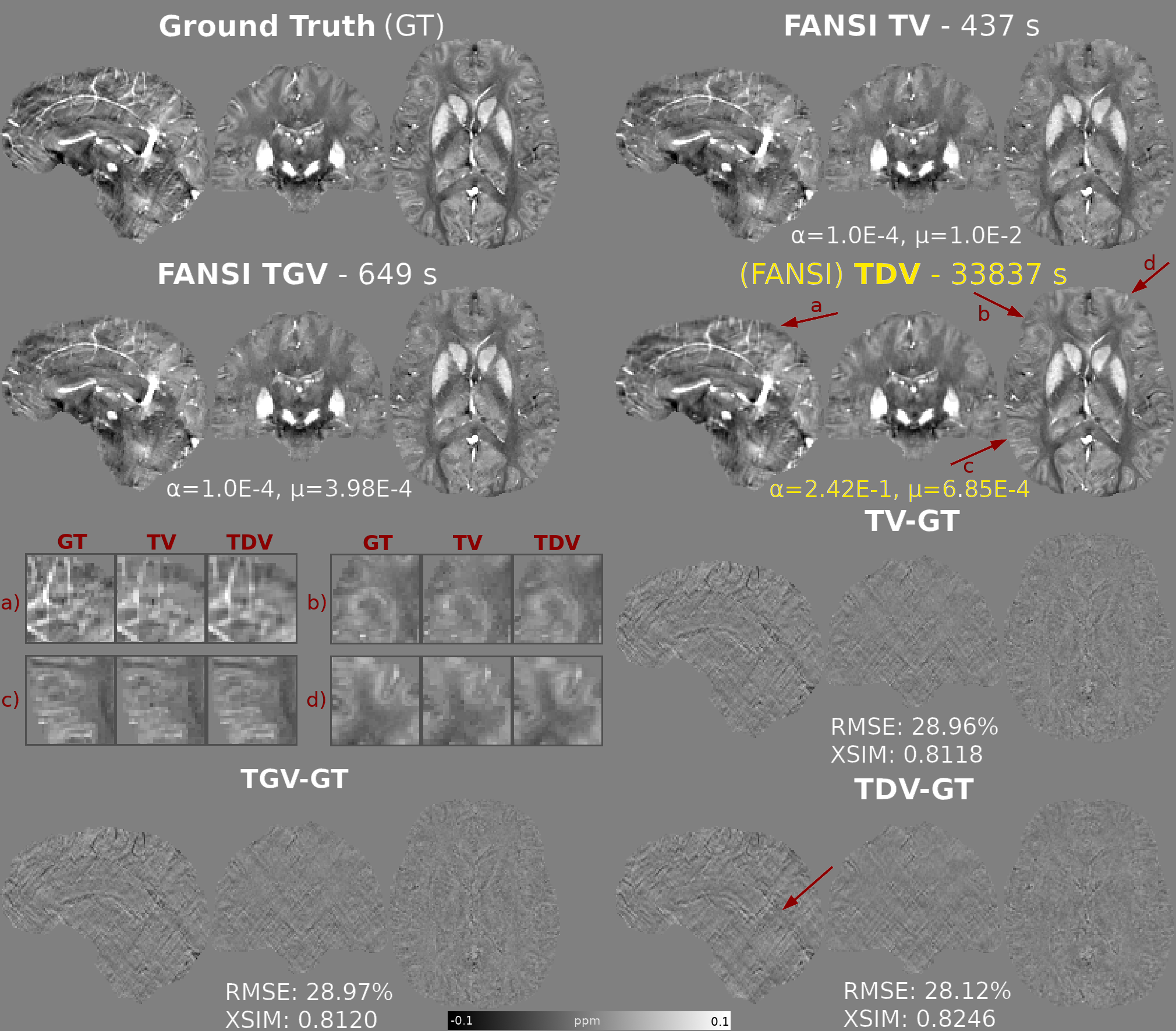
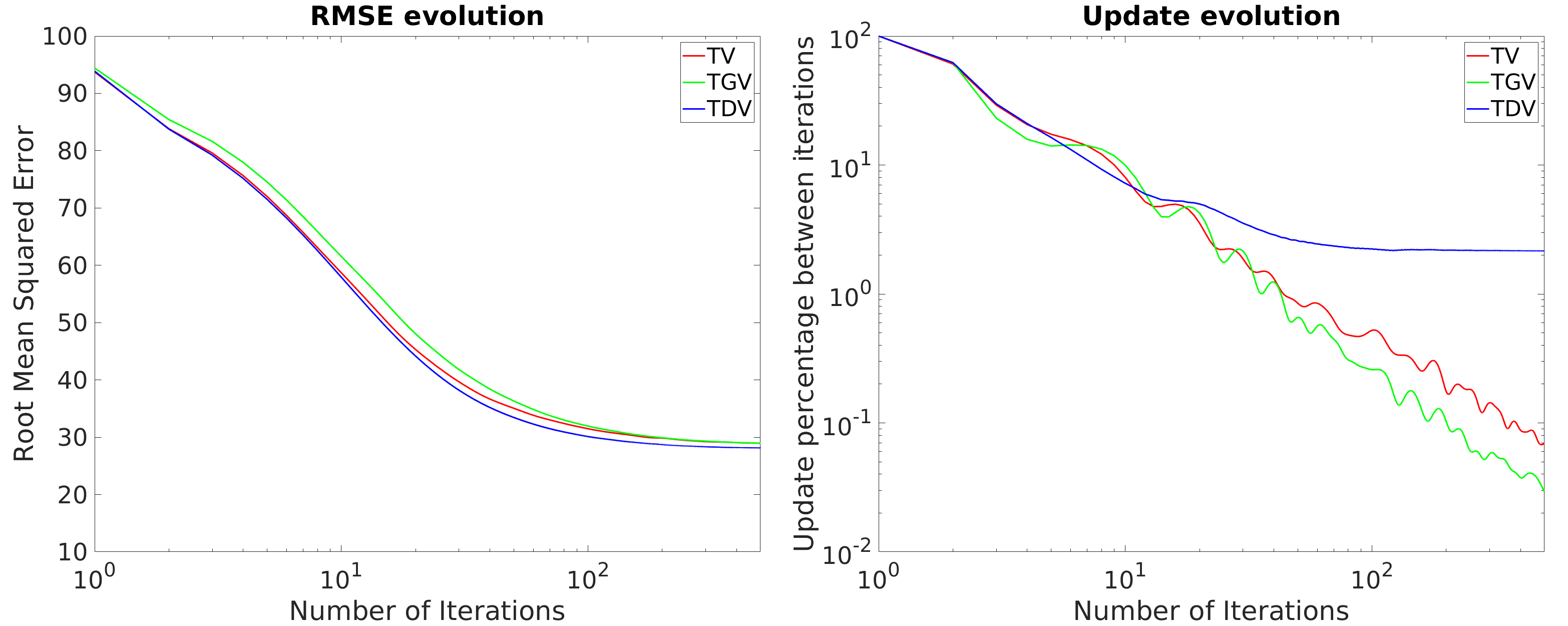
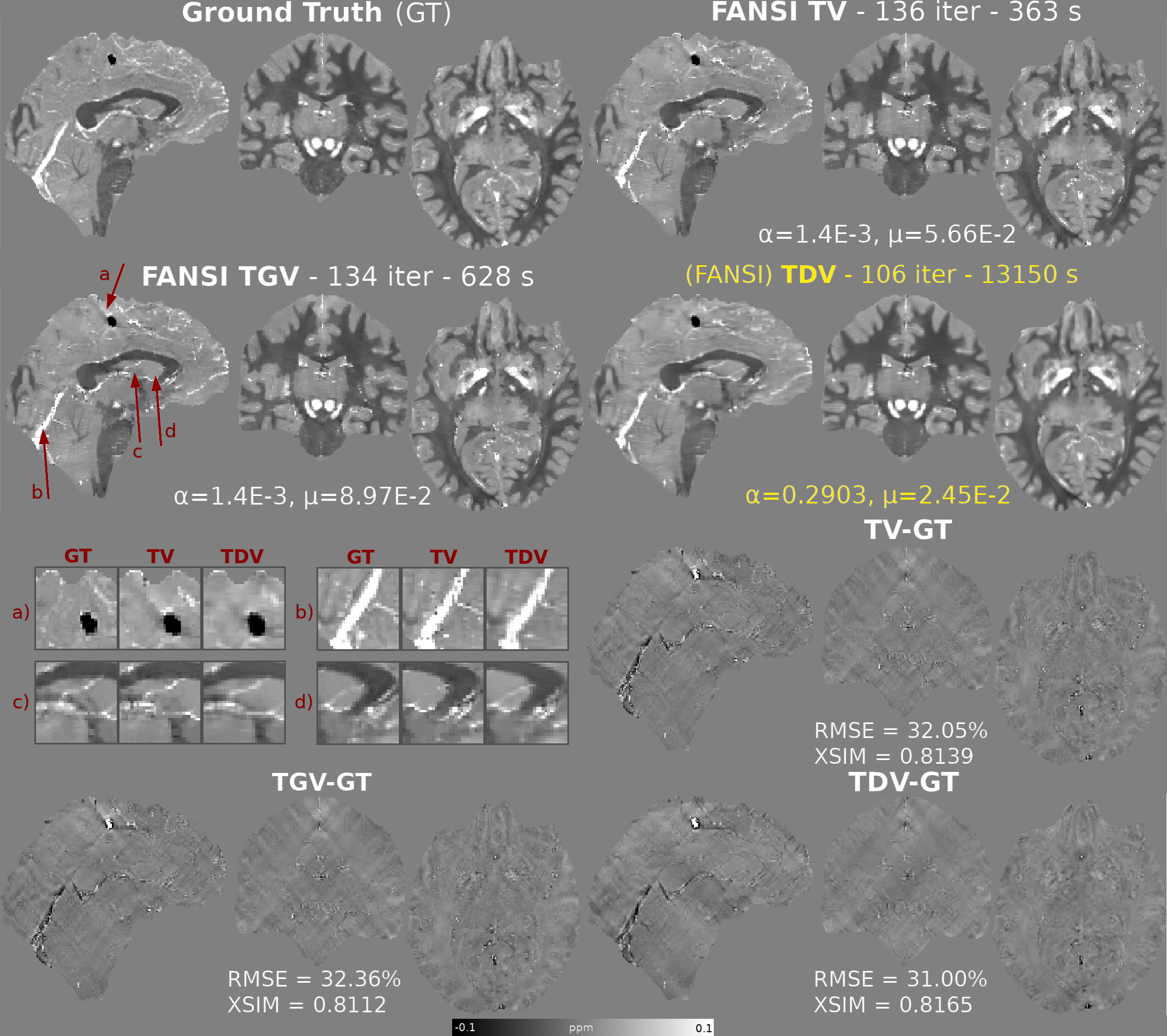
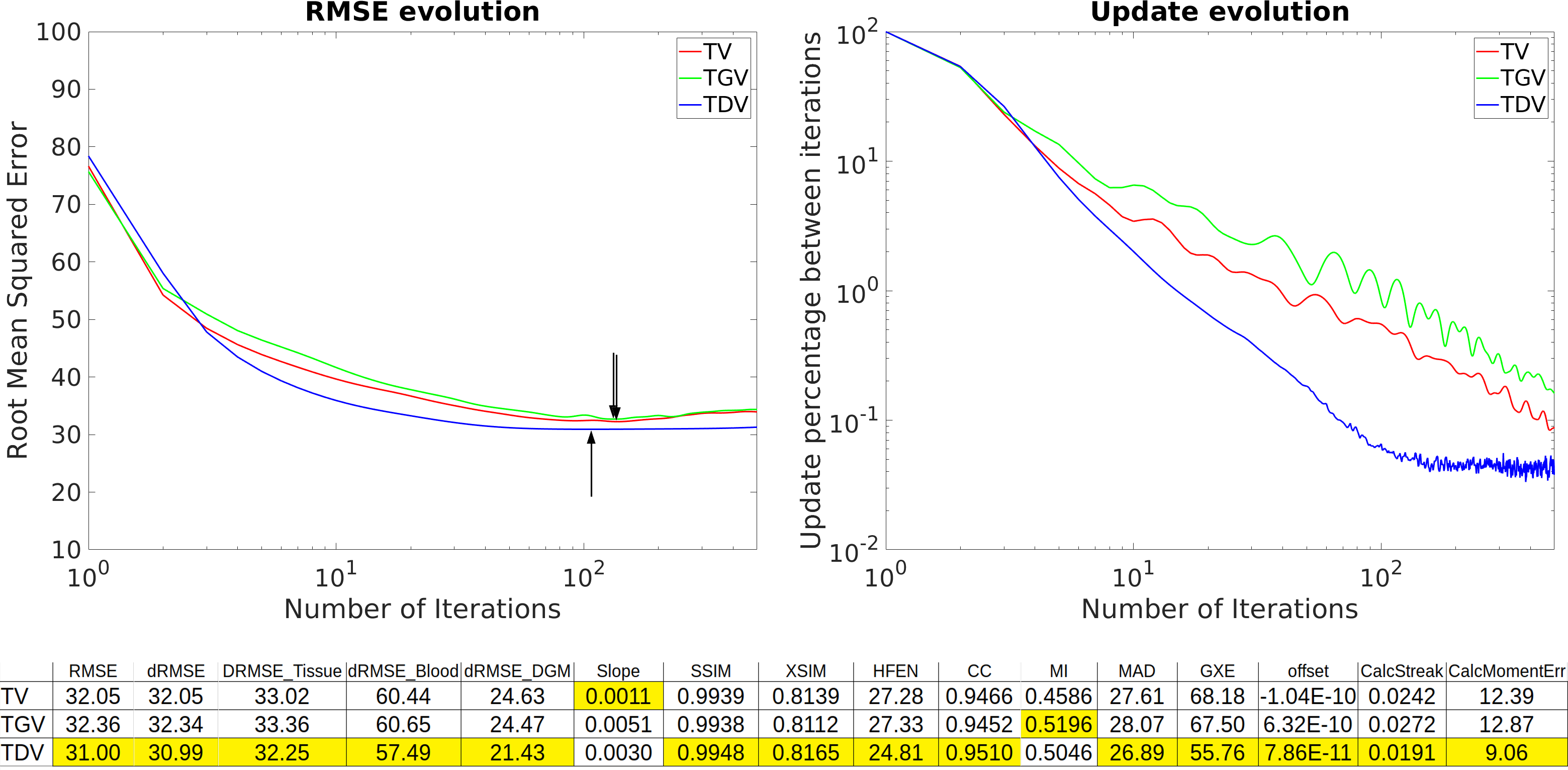
The pre-trained TDV network for 2D color images was extended to 3D images by inputting groups of three consecutive slices as red, green and blue channels of 2D color images, until the whole volume was denoised. We compared reconstructions obtained by TDV regularization with FANSI-TV⁵ (which achieved the best RMSE in RC2, Stage 2)⁷ and FANSI-TGV⁵. We used two synthetic brain models to compare reconstructions: 1) A forward simulation (SNR=100) from the COSMOS-based 2016 QSM Challenge dataset (RC1)¹⁵, and 2) the SIM2SNR1¹⁶ field map from RC2. We also compared the reconstructions in a healthy female volunteer scanned for another study¹⁷ at 3T (Achieva, Philips Healthcare, NL) using a 32-channel head coil and a 3D GRE sequence with 5 echoes, TE1/ΔTE/TR=3/5.4/29ms, flip angle=20°, matrix size = 240×240×144, and 1 mm3 isotropic voxels. Multi-echo combination was performed by nonlinear fitting⁴. Unwrapping was performed using SEGUE¹⁸. Background field removal was performed by the Laplacian Voundary Value (LBV)¹⁹ method and then by Weak Harmonics QSM (WH-QSM)²⁰ to remove any residual background fields. We used bespoke masking based on R2* maps to remove inflow effects in the reconstructions. The root mean squared error (RMSE), QSM-tuned structural similarity index²¹ (XSIM), and RC2-specific metrics⁷ were used to compare the phantom susceptibility maps.

RESULTS

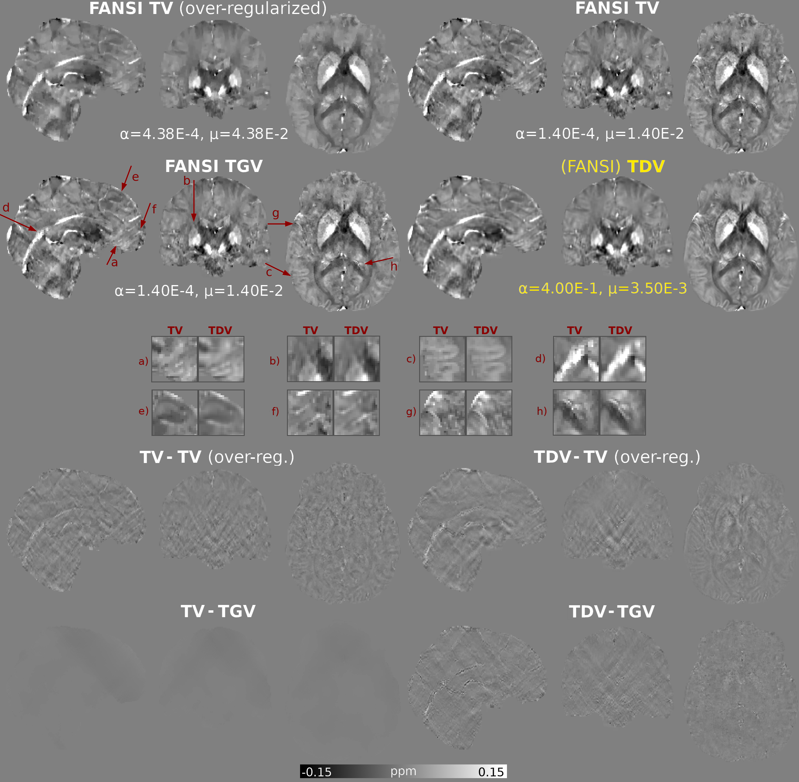
Optimal RMSE reconstructions and error maps using RC1 are shown in Figure 1. TDV shows better depiction of cortical areas (a-d) and less staircasing (a) and streaking artifacts (error maps) than TV and TGV. TDV converged with slightly fewer iterations than TV and TGV (Figure 2), achieving better RMSE and XSIM scores (Figure 1). TDV results in RC2 show better depiction of the veins (Figure 3, b-d) and streaking artifact suppression (a) relative to TV and TGV. TDV converged with fewer iterations and was more stable (Figure 4), performing better in almost all error metrics. In-vivo reconstructions are shown in Figure 5. TDV shows increased contrast in some deep structures and between white matter and grey matter (a-c), and some attenuation of noise and streaking near the vessels (d-h).

DISCUSSION

In all our experiments, optimal TV and TGV reconstructions are almost identical. TDV results show promising, albeit subtle, improvements over TV and TGV, despite the increased computation time. Our implementation is not optimal, and may be improved in terms of performance and computation time by retraining the TDV network with 3D data. Retraining may also target suppression of QSM streaking artifacts.

CONCLUSION

We have demonstrated that, even using a pre-trained network, Total Deep Variation denoising may be used for QSM and it achieved improved reconstructions compared to state-of-the-art TV and TGV regularized algorithms. Future TDV developments will focus on QSM-specific retraining and solver optimization.

Acknowledgements

Dr Carlos Milovic is supported by Cancer Research UK Multidisciplinary Award C53545/A24348. Dr Karin Shmueli is supported by European Research Council Consolidator Grant DiSCo MRI SFN 770939. We thank Dr. Anita Karsa for her MRI data and contributions.

References

1. Li L, Leigh JS. Quantifying arbitrary magnetic susceptibility distributions with MR. Magn Reson Med. 2004;51:1077-82

2. Kee Y, Liu Z, Zhou L, Dimov A, Cho J, de Rochefort L, Seo JK, Wang Y. Quantitative Susceptibility Mapping (QSM) Algorithms: Mathematical Rationale and Computational Implementations. IEEE Trans Biomed Eng. 2017;64:2531-2545

3. Kressler B, Rochefort L De. Nonlinear regularization for per voxel estimation of magnetic susceptibility distributions from MRI field maps. IEEE Trans Med Imaging 2010;29:273–281

4. Liu T, Wisnieff C, Lou M, Chen W, Spincemaille P, Wang Y. Nonlinear formulation of the magnetic field to source relationship for robust quantitative susceptibility mapping. Magn Reson Med. 2013;69:467-476

5. Milovic C, Bilgic B, Zhao B, Acosta-Cabronero J, Tejos C. Fast nonlinear susceptibility inversion with variational regularization. Magn Reson Med. 2018;80:814-821

6. Langkammer C, Bredies K, Poser B, Barth M, Reishofer G, Fan AP, Bilgic B, Fazekas F, Mainero C, Ropele S. Fast quantitative susceptibility mapping using 3D EPI and total generalized variation. Neuroimage 2015;111:622-630

7. QSM Challenge Committee. QSM Reconstruction Challenge 2.0: Design and Report of Results. BioRxiv 2020 doi:10.1101/2020.11.25.397695

8. Jung W, Bollmann S, Lee J. Overview of quantitative susceptibility mapping using deep learning: Current status, challenges and opportunities. NMR in Biomedicine. 2020;e4292

9. Hammernik K, Klatzer T, Kobler E, Recht MP, Sodickson DK, Pock T, Knoll F. Learning a variational network for reconstruction of accelerated MRI data. Magn Reson Med. 2018;79(6):3055-3071

10. Polak, D, Chatnuntawech, I, Yoon, J, et al. Nonlinear dipole inversion (NDI) enables robust quantitative susceptibility mapping (QSM). NMR Biomed. 2020;e4271

11. Kobler E, Effland A, Kunisch K, Pock T. Total Deep Variation for Linear Inverse Problems. Proceedings of the IEEE/CVF Conference on Computer Vision and Pattern Recognition (CVPR), 2020;7549-7558

12. Roth S, Black MJ. Fields of Experts. Int J Comput Vis 2009;82:205

13. Martin D, Fowlkes C, Tal D and Malik J. A database of human segmented natural images and its application to evaluating segmentation algorithms and measuring ecological statistics. Proceedings Eighth IEEE International Conference on Computer Vision. ICCV 2001, Vancouver, BC, Canada, 2001;2:416-423

14. Boyd S, Parikh N, Chu E, Peleato B, and Eckstein J. Distributed Optimization and Statistical Learning via the Alternating Direction Method of Multipliers. Foundations and Trends in Machine Learning, 2011;3:1–122

15. Langkammer C, Schweser F, Shmueli K, Kames C, Li X, Guo L, Milovic C, Kim J, Wei H, Bredies K, Buch S, Guo Y, Liu Z, Meineke J, Rauscher A, Marques JP, Bilgic B. Quantitative susceptibility mapping: Report from the 2016 reconstruction challenge. Magn Reson Med. 2018;79:1661-1673

16. Marques JP, Meineke J, Milovic C, Bilgic B, Chan K-S, Hedouin R, van der Zwaag W, Langkammer C, and Schweser F. QSM Reconstruction Challenge 2.0: A Realistic in silico Head Phantom for MRI data simulation and evaluation of susceptibility mapping procedures. bioRxiv 2020.09.29.316836; doi: https://doi.org/10.1101/2020.09.29.316836

17. Karsa A, Punwani S, and Shmueli K. The effect of low resolution and coverage on the accuracy of susceptibility mapping. Magn Reson Med. 2019; 81: 1833– 1848

18. Karsa A, Shmueli K. SEGUE: A Speedy rEgion-Growing Algorithm for Unwrapping Estimated Phase. IEEE Trans Med Imaging. 2019;38:1347-1357

19. Zhou D, Liu T, Spincemaille P, and Wang Y. Background field removal by solving the Laplacian boundary value problem. NMR Biomed, 2014;27:312-319

20. Milovic C, Bilgic B, Zhao B, Langkammer C, Tejos C, Acosta-Cabronero J. Weak-harmonic regularization for quantitative susceptibility mapping. Magn Reson Med. 2019;81:1399-1411

21. Milovic C, Tejos C, and Irarrazaval P. Structural Similarity Index Metric setup for QSM applications (XSIM). 5th International Workshop on MRI Phase Contrast & Quantitative Susceptibility Mapping, Seoul, Korea, 2019

Figures

Figure 1: Optimal reconstructions and error maps of COSMOS-based forward simulations (RC1) for all regularization methods (TDV, TV and TGV). A sagittal, coronal and axial slice are shown. All methods were terminated after 500 iterations. TDV shows better depiction of cortical areas and less staircasing and streaking artifacts (highlighted with red arrows) than TV and TGV and achieves better RMSE and XSIM scores. Detailed comparisons between TV and TDV are shown for each labeled region (a-d).

Figure 2: RMSE and update convergence for all regularization methods (TDV, TV and TGV) on the RC1 numerical phantom. The update convergence is defined as: $$$100||\chi_k-\chi_{k-1}||/||\chi_k||$$$) where k is the iteration number. TDV converges very slightly faster than TV and TGV.

Figure 3: Optimal reconstructions of the RC2 numerical phantom for all regularization methods (TDV, TV and TGV). TDV results show better depiction of the veins and streaking artifact suppression relative to TV and TGV (relevant areas highlighted with red arrows).

Figure 4: RMSE and update convergence for all regularization methods (TDV, TV and TGV) on the RC2 numerical phantom (Top). The update convergence is defined as: $$$100||\chi_k-\chi_{k-1}||/||\chi_k||$$$) where k is the iteration number. An extended set of RC2 error metrics for all methods is shown below. TDV converged faster and was more stable, performing better in almost all error metrics.

Figure 5: Optimal reconstructions (L-curve analysis) for TDV, TV and TGV in vivo. An over-regularized TV solution is also shown to facilitate assessment of streaking artifacts and the sharpness of fine details. Relative to TV and TGV, TDV shows larger differences for deep brain structures (due to increased contrast), and smaller differences for cortical areas (indicating stronger streaking artifact suppression). Areas highlighted with arrows (a-h) show that TDV clearly depicts vessels and other structures, while noise is supressed without noticeable artifacts.

Proc. Intl. Soc. Mag. Reson. Med. 29 (2021)

3979