3978
NeXtQSM - A complete deep learning pipeline for data-consistent quantitative susceptibility mapping trained with synthetic data1Centre for Advanced Imaging, The University of Queensland, Brisbane, Australia, 2ARC Training Centre for Innovation in Biomedical Imaging Technology, The University of Queensland, Brisbane, Australia, 3Siemens Healthcare Pty Ltd, Brisbane, Australia, 4High Field MR Center, Department of Biomedical Imaging and Image-Guided Therapy, Medical University of Vienna, Vienna, Austria, 5Department of Neurology, Medical University of Graz, Graz, Austria, 6School of Information Technology and Electrical Engineering, The University of Queensland, Brisbane, Australia
Synopsis
Deep learning based quantitative susceptibility mapping has shown great potential in recent years, outperforming traditional non-learning approaches in speed and accuracy in many applications. Here we aim to overcome the limitations of in vivo training data and model-agnostic deep learning approaches commonly used in the field. We developed a new synthetic training data generation method that enables the background field correction and a data-consistent solution of the dipole inversion to be learned using a variational network in one pipeline. NeXtQSM is a complete deep learning based pipeline for computing robust, fast and accurate quantitative susceptibility maps.
Introduction
Deep learning techniques have been applied to multiple problems in MRI and shown effectiveness in efficiently solving several problems such as dipole inversion for Quantitative Susceptibility Mapping (QSM)1,2 or background field correction3 to remove the effect of external sources (e.g., air-tissue interfaces). However, current deep learning QSM techniques have multiple shortcomings such as requiring in vivo training data, not incorporating data-consistency constraints and treating the background field correction and dipole inversion as separate problems. To address these problems, we propose NeXtQSM, a deep learning pipeline to solve the background field correction and dipole inversion in a data consistent fashion trained on synthetic data.Methods
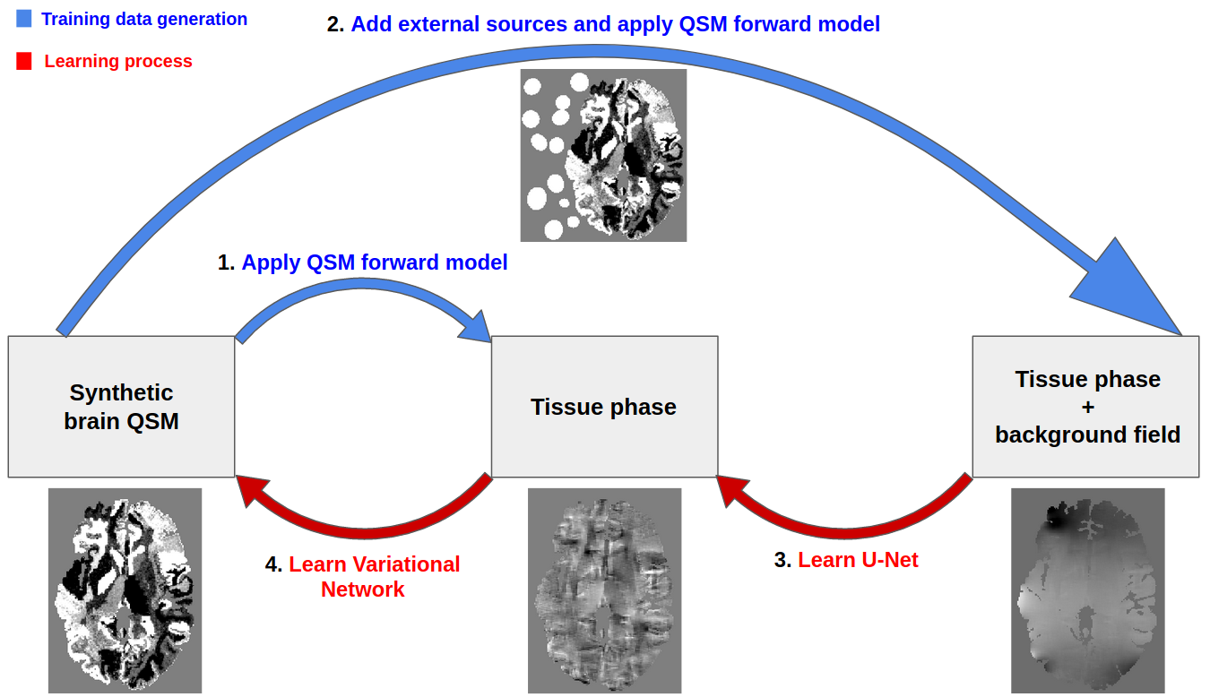
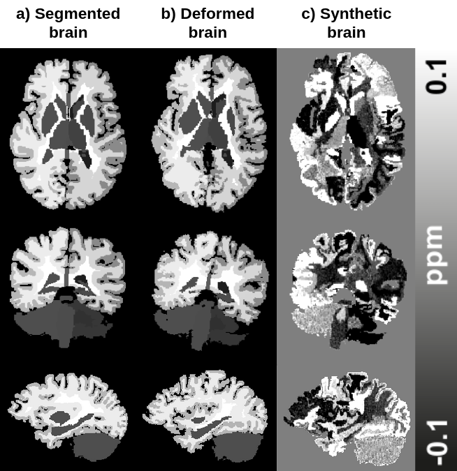
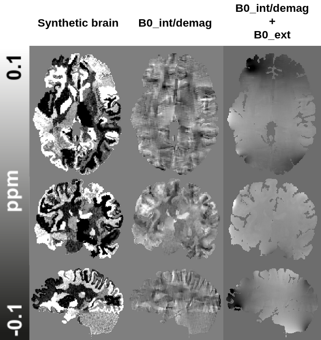
The pipeline (Fig. 1) is composed of two deep learning architectures trained together in an end-to-end fashion for solving background field removal and dipole inversion. In order to evaluate the performance of the pipeline, we used in vivo data from the QSM challenge 20164.Both models in the pipeline utilized realistic simulations of the physical properties of the problems and complex realistic structures. The synthetic data was based on the deformation of segmented brains using affine transformations and a Gaussian Mixture Model5, which substituted the class labels with randomly sampled intensities from a prior distribution (Fig. 2). The synthetic data was generated from 28 individuals’ MP2RAGE scans segmented using FreeSurfer v66. The training data generation consisted of applying the QSM forward operation to the FreeSurfer wmparc segmentation maps to simulate data with realistic properties. For the background field removal problem, external sources were simulated around the brain before convolving it with the QSM forward model (Fig. 1 & 3).
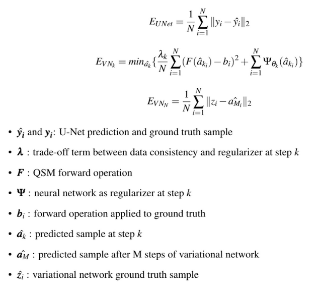
The first stage of the pipeline used a U-Net7 to learn the background field correction. The second stage used a variational network8,9 to enable a data-consistent solution of the QSM dipole inversion. This iterative hybrid model was derived from traditional variational methods, but instead of using a hand-crafted regularizer based on prior knowledge, a regularizer was learned from the data using convolutional neural networks. In addition to the learned prior term, its loss function also included a data consistency term, in our case the QSM forward model, which helps in applying the model to a variety of input data that would lead to unstable solutions in model-agnostic deep learning solutions.
The different loss functions used at each stage of the pipeline can be found in Fig. 4. Our variational network was composed of 7 iteration-steps, with a different shallow U-Net7 as a regularizer at each step. The training was done in an end-to-end fashion, on both the background field and dipole inversion architectures jointly. At each training epoch, 4500 synthetic brains were used to learn the problem.
Results
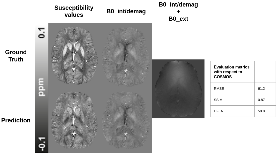
Fig. 5 shows the performance of the NeXtQSM when applied to the dataset from the QSM challenge 20164, where the QSM reconstruction is compared to the COSMOS ground truth. The results indicate that our synthetic training data captures both the geometrical and physical properties needed to train deep learning models, which are able to generalize to in vivo data. Using the metrics for the QSM challenge 20164, our pipeline achieves a score of 61.2 for RMSE, 0.87 for SSIM and 58.8 for HFEN with respect to the provided COSMOS ground truth.Discussion
Our pipeline is capable of learning the background field correction and dipole inversion from synthetic training data. We show that the trained networks generalize well to in vivo data of the QSM challenge. NextQSM performance is compared to the COSMOS ground truth and it is important to note that this is computed using multiple orientations, whereas our pipeline requires only one orientation for reconstructing the susceptibility map. Both architectures may be further improved using techniques used for image generation such as residual blocks10 to ease the learning process of deep architectures and generative adversarial networks11,12 to improve the visual quality of the predicted data.Conclusion
In conclusion, we presented NextQSM, a complete deep learning pipeline trained only on synthetic samples to solve QSM’s background field and dipole inversion steps in a data-consistent fashion.Acknowledgements
This research was undertaken with the assistance of resources and services from the Queensland Cyber Infrastructure Foundation (QCIF).References
1. Bollmann, S. et al. DeepQSM - using deep learning to solve the dipole inversion for quantitative susceptibility mapping. NeuroImage 195, 373–383 (2019).
2. Yoon, J. et al. Quantitative susceptibility mapping using deep neural network: QSMnet. NeuroImage 179, 199–206 (2018).
3. Bollmann, S. et al. SHARQnet – Sophisticated harmonic artifact reduction in quantitative susceptibility mapping using a deep convolutional neural network. Z. Für Med. Phys. (2019) doi:10.1016/j.zemedi.2019.01.001.
4. Langkammer C, Schweser F, Shmueli K, Kames C, Li X, Guo L, Milovic C, Kim J, Wei H, Bredies K, Buch S, Guo Y, Liu Z, Meineke J, Rauscher A, Marques JP, Bilgic B. Quantitative susceptibility mapping: Report from the 2016 reconstruction challenge. Magn Reson Med. 2018 Mar;79(3):1661-1673. doi: 10.1002/mrm.26830. Epub 2017 Jul 31. PMID: 28762243; PMCID: PMC5777305.
5. Billot, B. et al. A Learning Strategy for Contrast-agnostic MRI Segmentation. ArXiv200301995 Cs Eess (2020).
6. Whole Brain Segmentation: Automated Labeling of Neuroanatomical Structures in the Human Brain, Fischl, B., D.H. Salat, E. Busa, M. Albert, M. Dieterich, C. Haselgrove, A. van der Kouwe, R. Killiany, D. Kennedy, S. Klaveness, A. Montillo, N. Makris, B. Rosen, and A.M. Dale, (2002). Neuron, 33:341-355.
7. Ronneberger, O., Fischer, P. & Brox, T. U-Net: Convolutional Networks for Biomedical Image Segmentation. in Medical Image Computing and Computer-Assisted Intervention – MICCAI 2015 234–241 (Springer, Cham, 2015). doi:10.1007/978-3-319-24574-4_28.
8. Hammernik, K. et al. Learning a variational network for reconstruction of accelerated MRI data: Magn. Reson. Med. 79, 3055–3071 (2018).
9. Kames, C., Doucette, J. & Rauscher, A. ProxVNET: A proximal gradient descent-based deep learning model for dipole inversion in susceptibility mapping. in Proc. Intl. Soc. Mag. Reson. Med. 28 3198 (2020).
10. He, K., Zhang, X., Ren, S., Sun, J. (2016). Deep residual learning for image recognition. In IEEE proceedings of international conference on computer vision and pattern recognition (CVPR).
11. Goodfellow, I.J., Pouget-Abadie, J., Mirza, M., Xu, B.,Warde-Farley, D., Ozair,S., Courville, A., Bengio, Y.: Generative adversarial networks (2014)
12. P. Isola, J.-Y. Zhu, T. Zhou, and A. A. Efros, Image-to-image translation with conditional adversarial networks, 2017 IEEE Conference on Computer Vision and Pattern Recognition (CVPR),pp. 5967–5976, 2017.Figures