Introduction

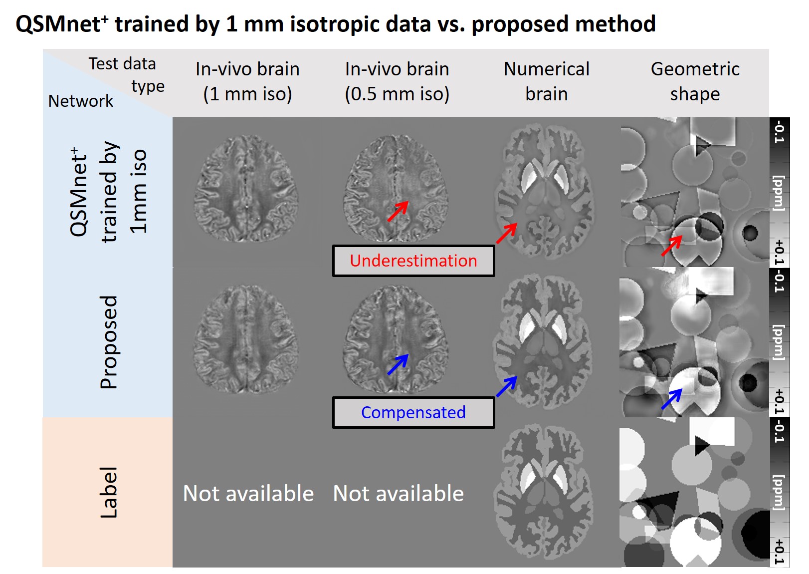
Recently, deep neural networks have shown great potential in quantitative susceptibility mapping (QSM).^1-4 Although a few studies have shown out-performance of deep learning-based QSM compared to conventional algorithms, generalization of the network to test data with different characteristic to the training data is limited.^5,6 In particular, recent deep learning-based QSM (QSMnet⁺) shows unexpected underestimation patterns in a few image types (Figure 1). To understand the source of this underestimation, we explore the effects of the spatial gradient of training images in deep learning-based QSM. The spatial gradient is a metric for the spatial variation of images.^7,8 The experiment was performed by comparing the networks, which were trained on susceptibility maps with different spatial gradients.

Methods

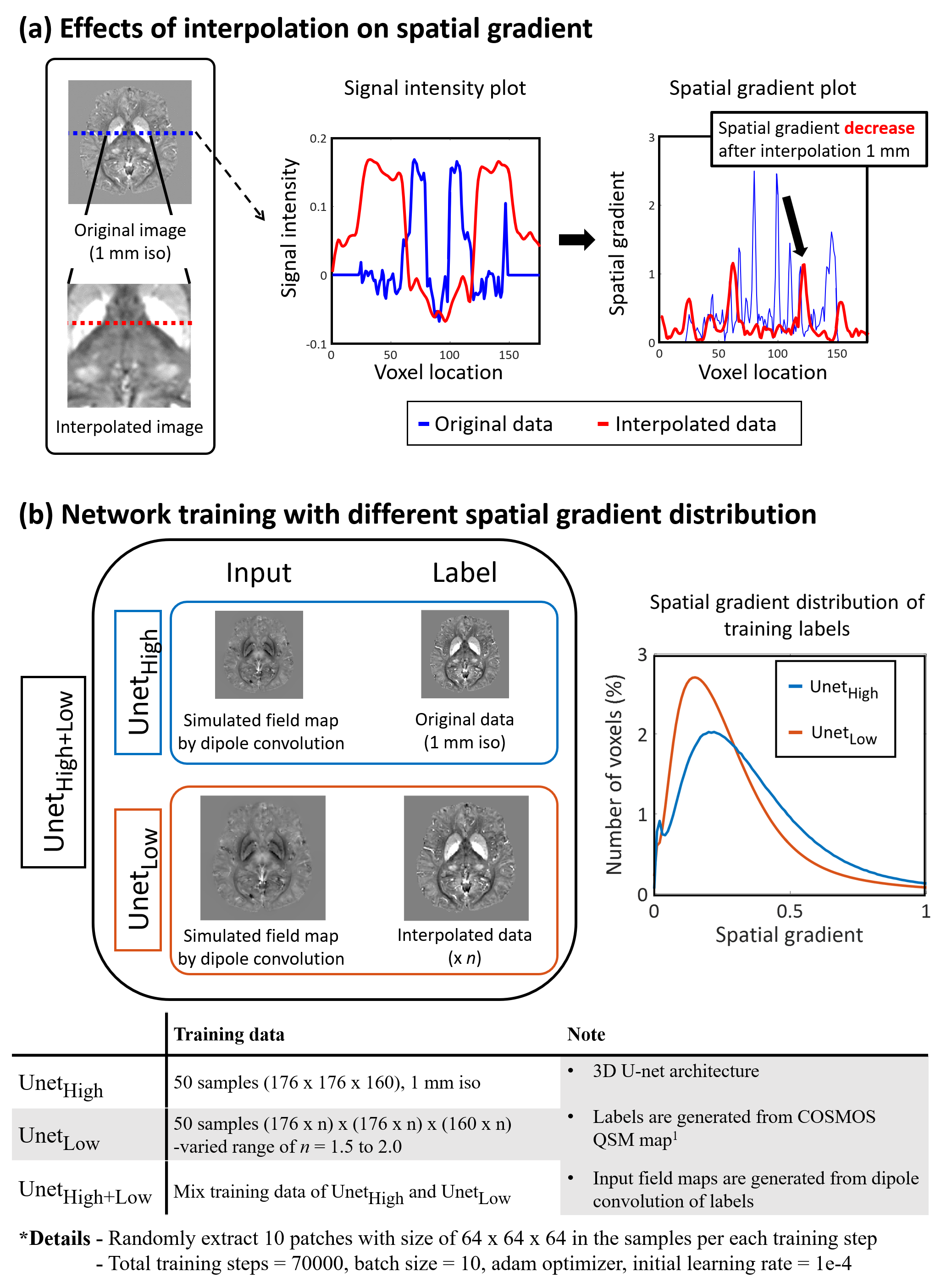
[Network training with different spatial gradient]
To explore the spatial gradient of the susceptibility maps as one factor for generalization of the network, the spatial gradient map is calculated using 3D-Sobel filter,⁷ which measures the numerical gradient of an image, as follows:$$g_{i}=s_{i}*\chi \,\,\,\,\,where\,\,\, i = x,y,and,z\,\,\,\,\,\,[Eq.1]$$ $$G=\sqrt{g_{x}^2+g_{y}^2+g_{z}^2}\,\,\,\,\,\,\,[Eq.2]$$where g_i is spatial gradient map of dimension i, s_i is Sobel filter value of dimension i, * is convolution operator, χ is susceptibility map, G is total spatial gradient map.

For demonstration, we trained two types of networks with different spatial gradient distributions: Unet_High and Unet_Low. Additionally, we trained Unet_High+Low by combining training data of Unet_High and Unet_Low to evaluate the performance of data augmentation. All networks were trained by labels as susceptibility maps, and inputs as dipole convolution of these labels. For Unet_High, susceptibility maps for labels were set from existing 1mm-isotropic COSMOS-QSM maps (QSMnet dataset).¹ To generate low spatial gradient training data for Unet_Low, sinc-interpolation was performed in the COSMOS-QSM maps. The effects of interpolation on spatial gradients are demonstrated in Figure 2a. All training details are summarized in Figure 2b. In each network, the histogram of the spatial gradient distributions of training data was estimated (Figure 2b).

[Evaluation]
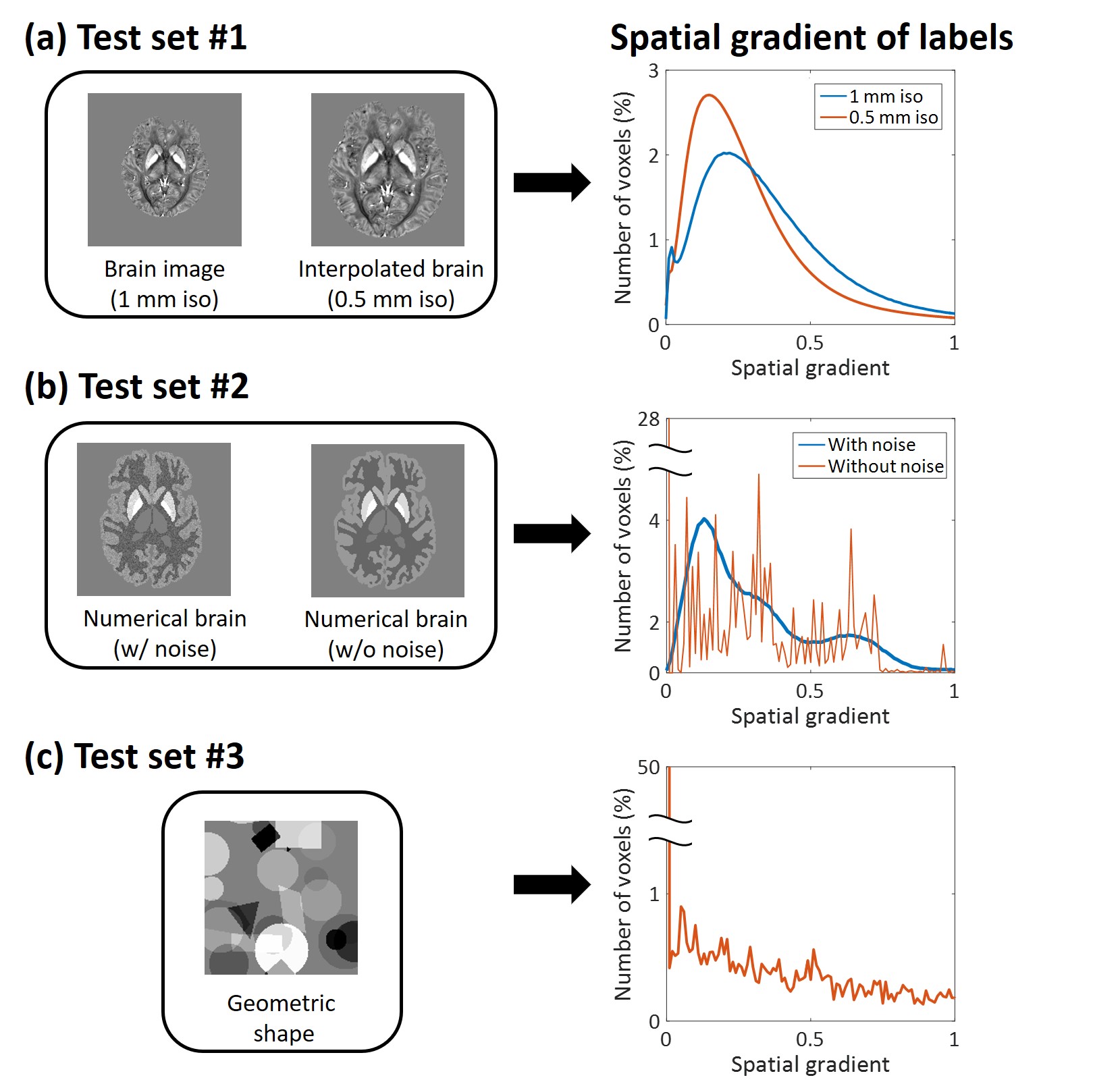
To evaluate the effects of spatial gradients on network performance, three networks were developed and applied to three different types of test data: brain images, numerical brain,⁹ and geometric shapes. First, the brain image dataset was generated from the QSMnet test dataset. Test dataset was generated in two different resolutions (0.5/1mm isotropic) in the same way as generating the training dataset (i.e.,sinc-interpolation). The second dataset was generated from the numerical brain. To test the networks in high spatial gradient images, additional numerical brain was generated by adding Gaussian noise. Lastly, to test the networks in low spatial gradient, geometric shapes were generated. All test data are summarized in Figure 3 including the histograms of the spatial gradients of the susceptibility maps. In all reconstructions, NRMSE with respect to the ground-truth was estimated.

Additionally, to test the networks in high-resolution brain images without interpolation, in-vivo brain images with 0.5mm-isotropic resolution were acquired at 7T using multi-echo gradient-echo sequence with the following parameters: TE=4.7:5.2:25.5ms/TR=36ms and matrix size=384x384x160. An ROI analysis is performed in low spatial gradient regions, which is manually segmented.

Results

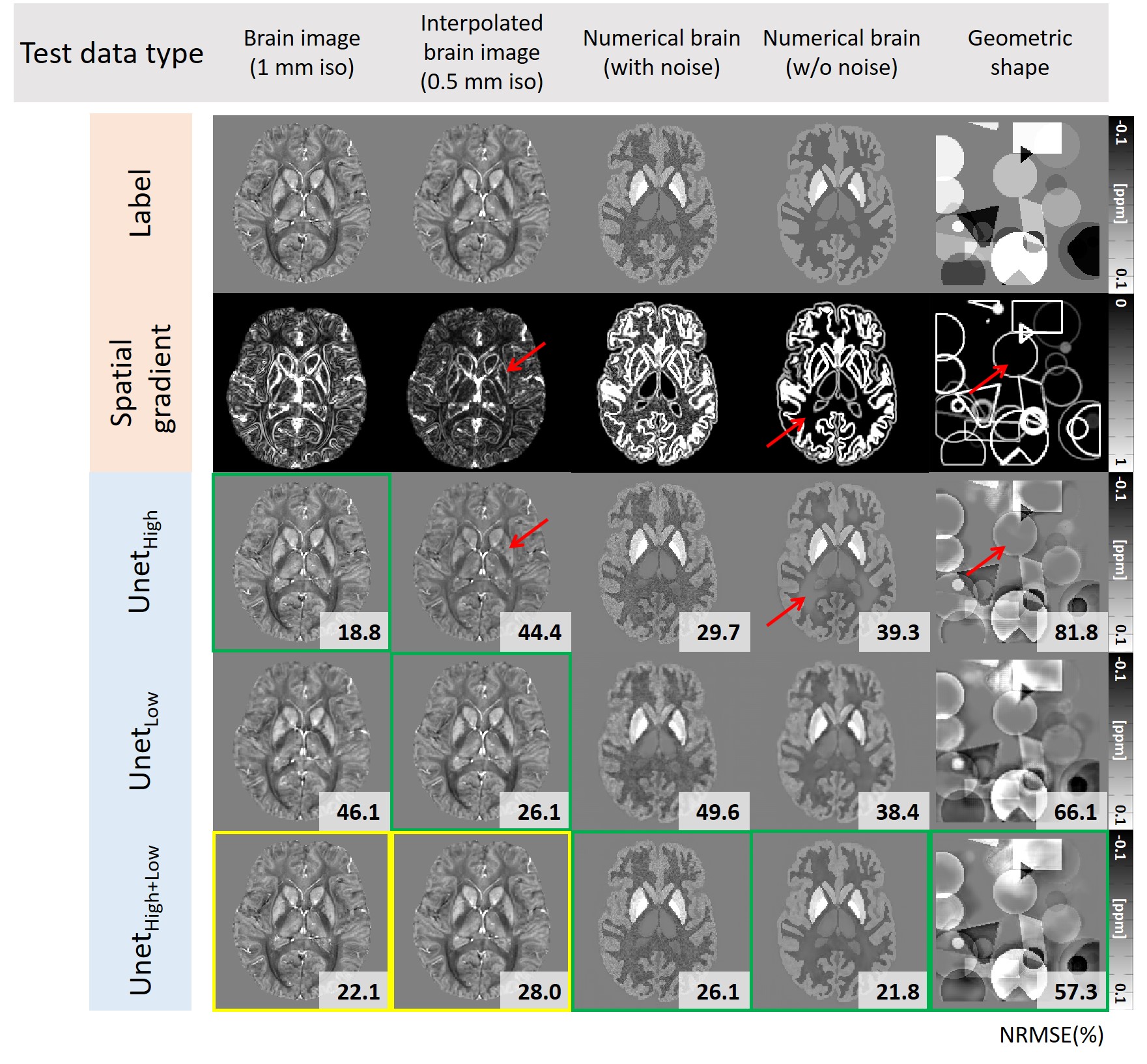
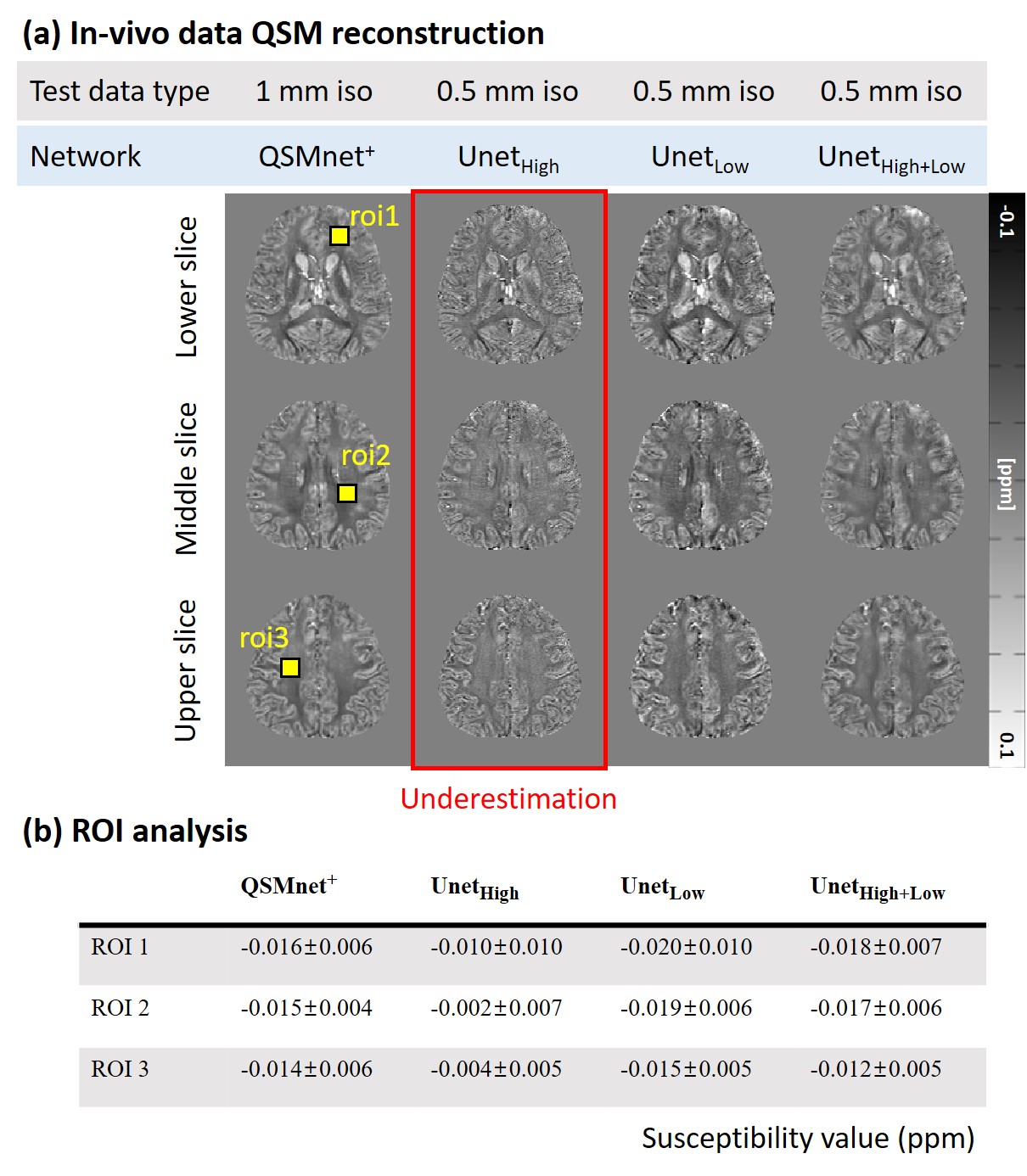
Figure 4 shows the QSM maps of the five inputs (brain images with 0.5mm and 1mm resolution, numerical brain with/without noise, and geometric shapes) reconstructed by three networks (Unet_High, Unet_Low, and Unet_High+Low). The first-two rows show the labels and the corresponding spatial gradient maps. The best performance is highlighted by green boxes with NRMSE in the right corner. As highlighted by red arrows, Unet_High shows underestimation in the low spatial gradient regions (0.5mm brain, numerical brain without noise, and geometric shapes) similar to Figure 1. This underestimation of Unet_High is reduced in 1mm brain or numerical brain with noise, which have higher spatial gradients. On the other hand, when the network was trained with low spatial gradients (Unet_Low), the underestimations in low spatial gradient regions (0.5mm brain, numerical brain without noise, and geometric shapes) are reduced as demonstrated by lower NRMSEs than the results of Unet_High. These outcomes suggest that the network performance is degraded when the spatial gradient distribution of the training data is different to the test data. Furthermore, data augmentation using the interpolated data (Unet_High+Low) demonstrates improved performance for all inputs as shown in the last row (yellow and green boxes), confirming the validity of the data augmentation approach for network generalization.

Figuer 5a shows the QSM maps of 0.5mm in-vivo brain reconstructed by Unet_High, Unet_Low, and Unet_High+Low. The results are compared with QSMnet⁺ reconstruction in 1mm resolution as a reference. As highlighted by the red box, Unet_High shows considerable underestimation compared to other networks. When the ROI analysis is performed, such underestimation is demonstrated in Figure 5b, reporting the mean/standard deviation of susceptibility values in the ROIs. The results suggest that the spatial gradient is an important consideration to the generalization of deep learning-based QSM for various resolutions.

Discussion and Conclusion

In this study, we demonstrate that deep-learning based QSM shows performance degradation when the spatial gradients of the training dataset is different from the test data. Particularly, the underestimations are consistently observed when the test data have lower spatial gradients than the training data. Using the training data with augmented spatial gradient distributions may improve deep learning-based QSM performance to work for a wide range of resolutions.

Acknowledgements

This research was supported by the National Research Foundation of Korea (NRF) grant funded by the Korea government (MSIT) (NRF-2019M3C7A1031994 and NRF-2018R1A2B3008445).