Introduction

Deep Learning (DL) methods are increasingly applied to Quantitative Susceptibility Mapping (QSM). Previously published articles have shown that, e.g., the dipole inversion and the background field correction in QSM can be solved with convolutional DL networks, even by training on synthetically generated data^1-3.
In QSM, the frequency of a voxel $$$f_B(\vec{r})$$$ is commonly approximated as a convolution between the dipole kernel $$$d(\vec{r})$$$, and the magnetic susceptibility $$$\chi(\vec{r})$$$¹:
$$f_B(\vec{r})=\frac{\gamma}{2\pi}B_0\cdot{}(d(\vec{r})*\chi(\vec{r})),\tag{Eq. 1}$$

where $$$\gamma$$$ is the gyromagnetic ratio and $$$*$$$ denotes the 3D-convolutional operator.

In most regions outside the brain, fat is present and Eq. 1 must be extended to account for its chemical shift. Here the complex gradient echo (GRE) signal $$$S(\vec{r},TE)$$$ depends on the voxel location $$$\vec{r}$$$ and the echo time TE can be modeled as:

$$S(\vec{r},TE)=\exp(2\pi i \cdot f_B(\vec{r})\cdot TE)\cdot\left(\rho_W(\vec{r})+\rho_F(\vec{r})\cdot\sum_{n=1}^N \alpha_n\cdot \exp(2 \pi i\cdot f_{F,n}\cdot TE)\right),\tag{Eq. 2}$$
with $$$\rho_W(\vec{r})$$$ and $$$\rho_F(\vec{r})$$$ the water and fat amplitude, $$$\alpha_n$$$ the relative amplitudes of the known frequency shifts $$$f_{F,n}$$$ of a multi fat peak spectrum⁴.
In this study, we propose a DL method for an integrated fat water separation, background field removal and dipole inversion to extend the use of DL QSM in regions outside the central nervous system (CNS).

Methods

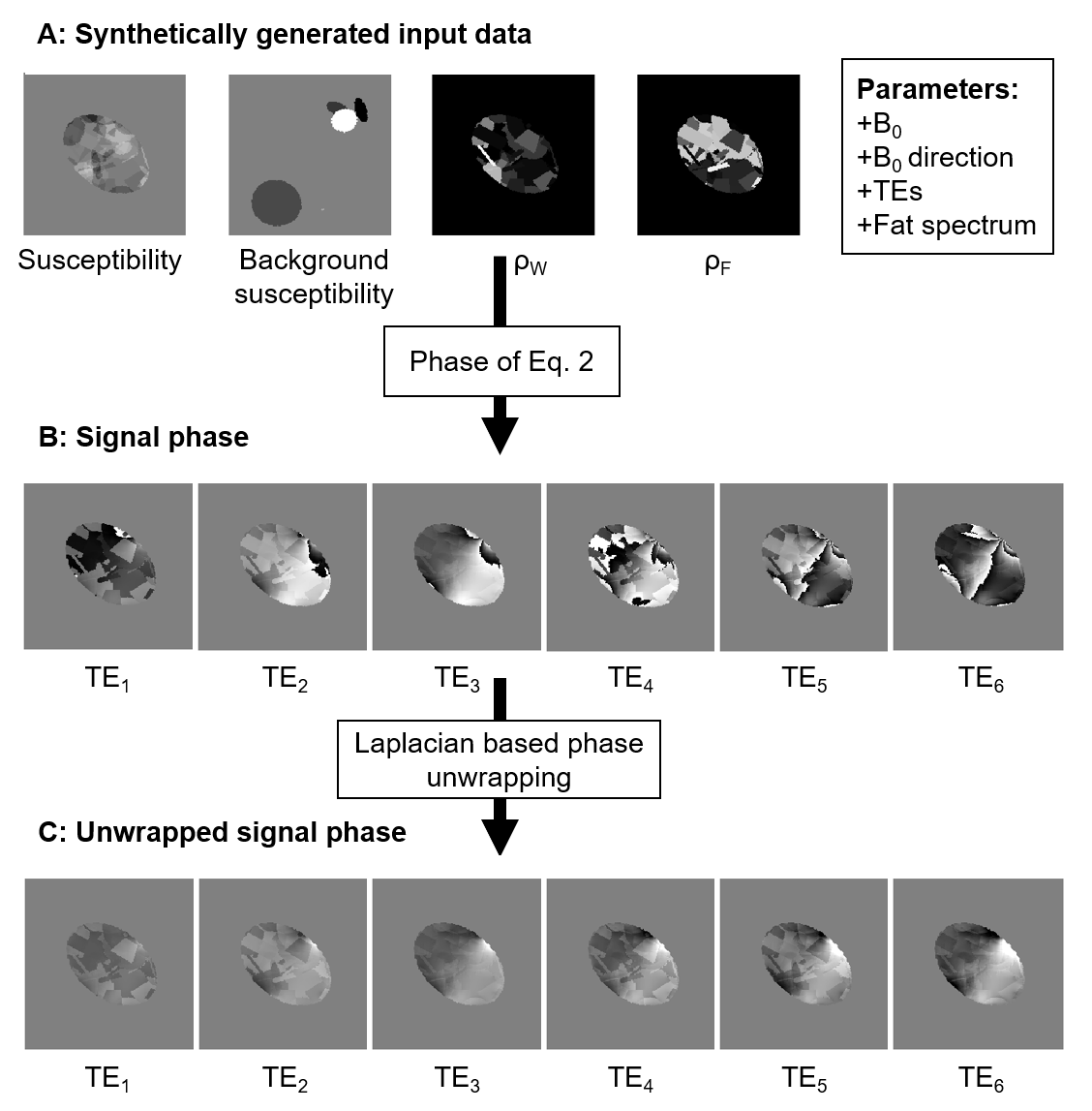
Synthetic data:
Synthetic 3D phase data was generated by simulating 300-400 cubes and ellipsoids with a randomly assigned magnetic susceptibility, fat $$$\rho_F(\vec{r})$$$ and water $$$\rho_W(\vec{r})$$$ amplitude.
The used parameter ranges were: $$$\rho_F(\vec{r})$$$ and $$$\rho_W(\vec{r}) \in [0,1]$$$ and $$$\chi(\vec{r})$$$ was randomly picked from a gaussian distribution with zero mean and 0.25 ppm standard deviation.
Background fields were simulated outside a random sized ellipsoidal region-of-interest (ROI) with a standard deviation of 12 ppm. In total, 180 3D data sets were created with a matrix size of $$$192\times 192 \times 192$$$, each employing a commonly used six peak fat model⁵. The magnetic field strength was set to $$$B_0 = 1.5\;\mathrm{T}$$$ and Eq. 2 was applied for six echo times at $$$TE = (2.8/5.82/8.84/11.86/14.88/17.89)\;\mathrm{ ms}$$$. The signal in the background ROI was set to zero.

Figure 1A shows the simulated susceptibility distribution, $$$\rho_W(\vec{r})$$$ and $$$\rho_F(\vec{r})$$$ of a representative data set. Subsequently, the signal phase of the complex signal was calculated (Fig. 1B). To overcome phase wraps, Laplacian-based phase unwrapping⁶ was applied to the signal phase (Fig. 1C).
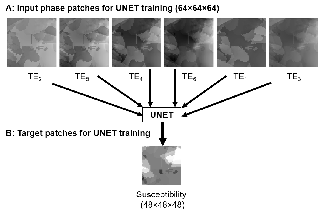
Of each of the 180 data sets, 50 patches (matrix size = $$$64\times64\times64$$$) were randomly cropped, resulting in a total of 9000 patches, which were used to train a convolutional neural network.

Neural network architecture:
A UNET⁷ was implemented, with the same architecture as the generator described in ⁸ with six inputs at the input layer. Parameters were as follows: Adam optimizer (learning rate = 0.0005, beta1 = 0.5, beta2 = 0.999), batch size = 10. As a loss function, the L2 loss was chosen.
The network was trained for 43 h on a NVIDIA GeForce RTX 2080 GPU with 8 GB of memory.
$$$64\times64\times64$$$ patches of the unwrapped phase were taken as input and the respective $$$48\times48\times48$$$ patches of the susceptibility distribution as target.
Figure 2 shows a set of input unwrapped phase and target susceptibility patches for the UNET.

In vivo MRI measurements:
To test the convolutional neural network on in vivo data, knee and pelvis phase data of two healthy male volunteers were acquired. All measurements were performed at a 1.5T Siemens Magnetom Sola by using a GRE-sequence with a voxel size of $$$1\times1\times1$$$ (interpolated to $$$1\times1\times2$$$ and TEs equal to the simulated data).

Conventional QSM processing:
To compare the proposed DL method to a commonly used fat water separation QSM pipeline, a graphcut algorithm was applied⁴ with the same fat peaks as in the simulated data. To eliminate background fields, V-SHARP⁹ was used. Finally, susceptibility maps were obtained by using STAR-QSM¹⁰. Furthermore, susceptibility maps without fat water separation were reconstructed by applying the Laplacian-based phase unwrapping algorithm⁶, before V-SHARP.

Results

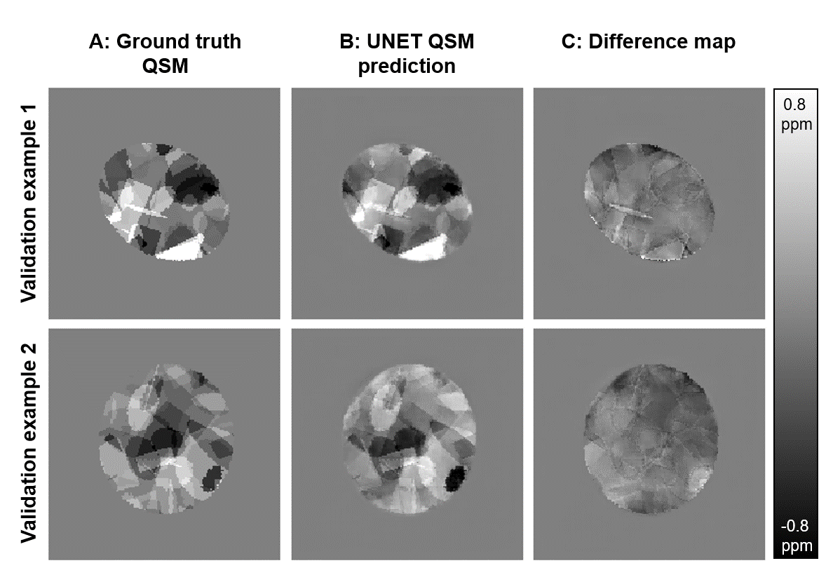
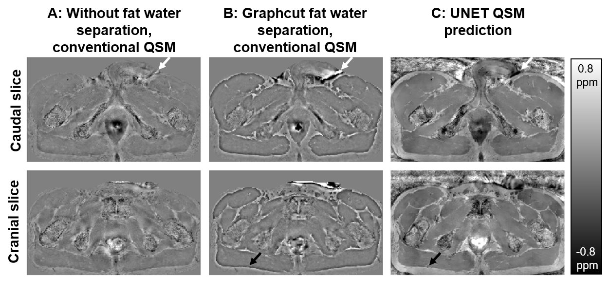
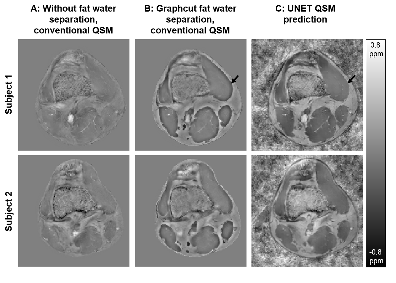
Figure 3 shows two representative examples of validation data evaluation, which were generated the same way as the training data, but not part of the UNET training.

Figures 4 and 5 show susceptibility maps of the male pelvis and of the knee respectively created by a conventional QSM pipeline without fat water separation (A), processed by a graphcut fat water separation algorithm with a conventional QSM pipeline (B) and the prediction of the proposed UNET (C).

Discussion

Our proposed UNET QSM reconstruction allows the reconstruction of high-quality susceptibility maps outside the brain. The level of apparent artifacts, e.g., near background sources (white arrows in Fig. 4) or at the boundary between fat and muscle (black arrows in Fig. 4 and 5) is reduced compared to a conventional fat water separation QSM pipeline.

Applying the trained network to data can be achieved in a few seconds and a mask generation for background field removal is not necessary, which increases the practicability.

The method can be adapted and trained to individual sequence and scanner parameters (B₀, B₀-direction, TEs and fat spectrum) within two days.

Conclusion

Deep learning based QSM reconstruction trained solely with synthetic data is well-suited to rapidly reconstruct high quality susceptibility maps in the presence of fat without the need of masking for background field removal.

Acknowledgements

The financial support by the Deutsche Forschungsgemeinschaft is gratefully acknowledged (grant DFG LA 2804/12‐1). We thank the Imaging Science Institute (Erlangen, Germany) for providing us with measurement time.