3970

Studying magnetic susceptibility, microstructural compartmentalisation and chemical exchange in a formalin-fixed, whole-brain specimen

Kwok-Shing Chan¹, Jeroen Mollink², Jenni Schulz¹, Anne-Marie van Cappellen van Walsum², and José P. Marques¹
¹Donders Institute for Brain, Cognition and Behaviour, Radboud University, Nijmegen, Netherlands, ²Department of Medical Imaging, Anatomy, Donders Institute for Brain, Cognition and Behaviour, Radboud University Medical Center, Nijmegen, Netherlands

Synopsis

In this work, we study the feasibility of using formalin-fixed post-mortem specimen to investigate MRI phase contrast in brain tissue. Despite the magnetic susceptibility maps derived from in vivo and ex vivo imaging share similar contrasts, the non-susceptibility contributions on measured fields of ex vivo sample were clear affected by fixation process, and we found its microstructural compartmentalisation effect are also greatly reduced. Therefore, extra care has to be taken to directly translate ex vivo findings to in vivo applications.

Introduction

Conventional QSM algorithms incorporate the Lorentzian-sphere correction in the dipole field formulation used to compute magnetic susceptibility, $$$\chi$$$^1,2. Yet, frequency shifts, $$$f$$$, used to compute $$$\chi$$$, do not have contributions solely from magnetic susceptibility but also microstructure compartmentalisation^3,4 and proton exchange between water and macromolecules^5–7. Furthermore, various studies showed that $$$\chi$$$ in white matter (WM) is anisotropic^8,9. Ex vivo imaging can be beneficial to disentangle the size of these contributions as it provides increased flexibility in scan duration, number of acquisitions with different orientations in respect to B₀ and validation with histology. Despite various studies reported formalin fixation significantly altered brain quantitative MRI parameters^10–12, this is still the most common tissue fixation protocol. In this study, we set out to probe the feasibility of using a formalin-fixed specimen to understand the MRI phase contrast in human brain.

Methods

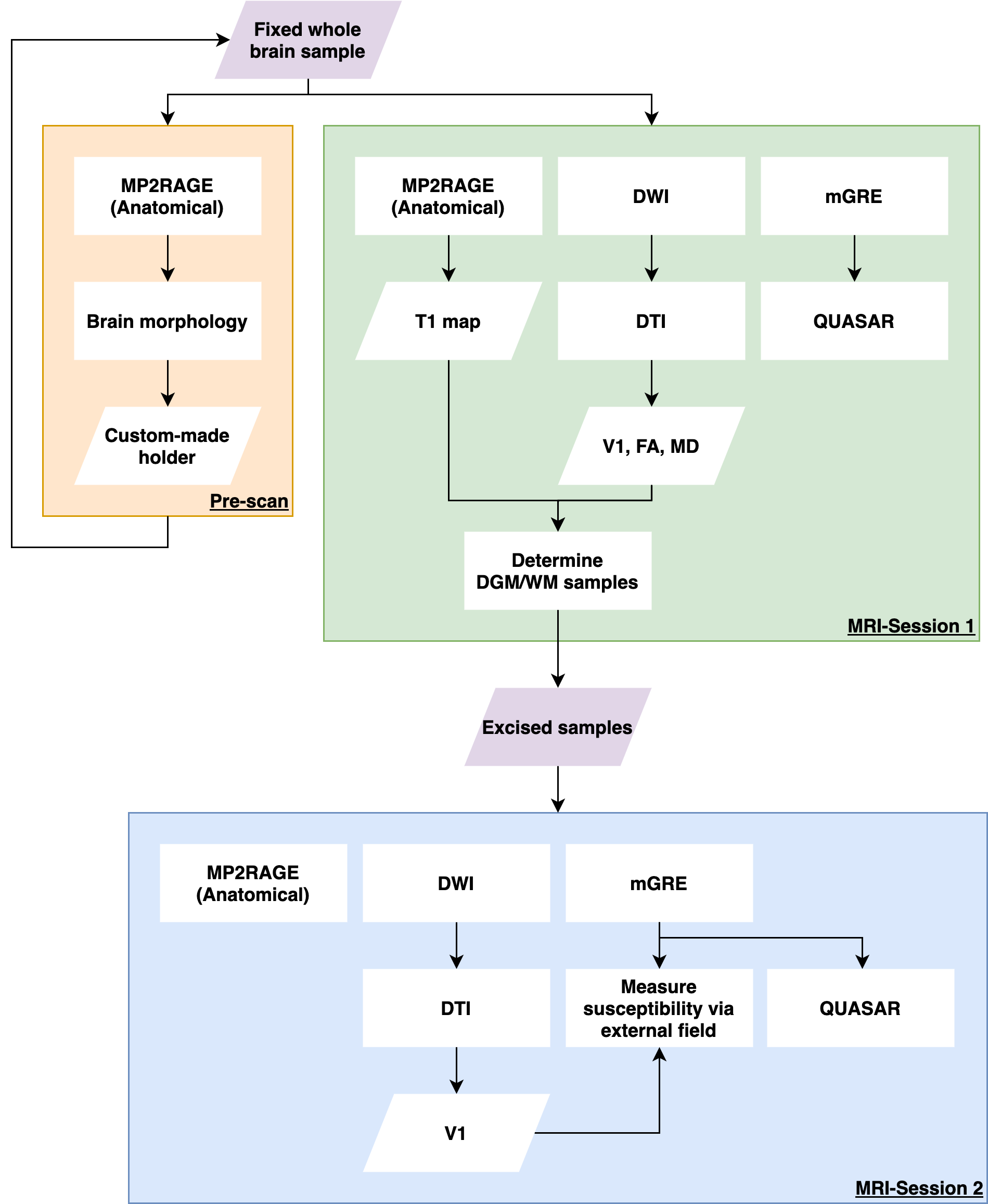
The experiment (described in Fig.1) included two imaging sessions at 3T (Siemens) using a 64-channel head coil. Firstly, a 5-month formalin-fixed post-mortem brain specimen was scanned inside a custom-made spherical holder¹³. The imaging protocol included:

MP2RAGE, TR/TI1/TI2=3000/311/1600ms, ɑ=4°/6°, res=1mm isotropic, Tacq=5min – adapted to sensitise MP2RAGE for T₁ between 0.25 and 1s;
DWI SE-EPI, SMS=3, res=1.6mm isotropic, TR/TE=3780/71.20ms, 2-shell (b=0/1250/2500s/mm²,17/120/120 measurements), NSA=20, Tacq=5.6hours.
Monopolar 3D mGRE: TR/TE=40/3.45:6.27:34.8ms (6 echoes), res=1mm isotropic, ɑ=20°, 10 orientations to B₀, Tacq=1.7hours;

10 WM ROIs were identified containing homogeneous tissue (volume≥64mm³ & DTI FA_ROI≥0.45) for further analysis. Tissues from these 10 locations and 2 in deep grey matter (DGM) were then excised, embedded in 1% agarose gel and scanned with the following protocol:

MP2RAGE, res=1mm isotropic, Tacq=5min;
DWI SE-EPI, res=1mm isotropic, TR/TE=15241/77.6, 2-shell (b=0/1250/2500s/mm²,17/120/120 measurements), NSA=9, Tacq=13.5hours.
Monopolar 3D mGRE: TR/TE=39.2/2.07:4.23:35.9ms (9 echoes), res=0.7mm isotropic, ɑ=15°, 10 orientations to B₀, Tacq=5.3hours;

All data were linearly registered to the GRE data that had its orientation adapted for better display on screen using ANTs¹⁴. Fieldmaps and tissue fields of all GRE data were computed using SEGUE¹⁵ phase unwrapping, optimum-weighted combination¹⁶ and LBV¹⁷ in SEPIA¹⁸. Subsequently, bulk isotropic magnetic susceptibility ($$$\chi$$$) and the field generated by non-susceptibility contributions ($$$f_{\rho}$$$) were computed using QUASAR¹⁹ adapted for multi-orientations:
$$f_{N}=d_{N}\ast\chi+f_{\rho}[Eq.1]$$
where $$$f_{N}$$$ and $$$d_{N}$$$ are the tissue field and the unit dipole associated with the acquisition at orientation N and $$$\ast$$$ is the convolution operator.

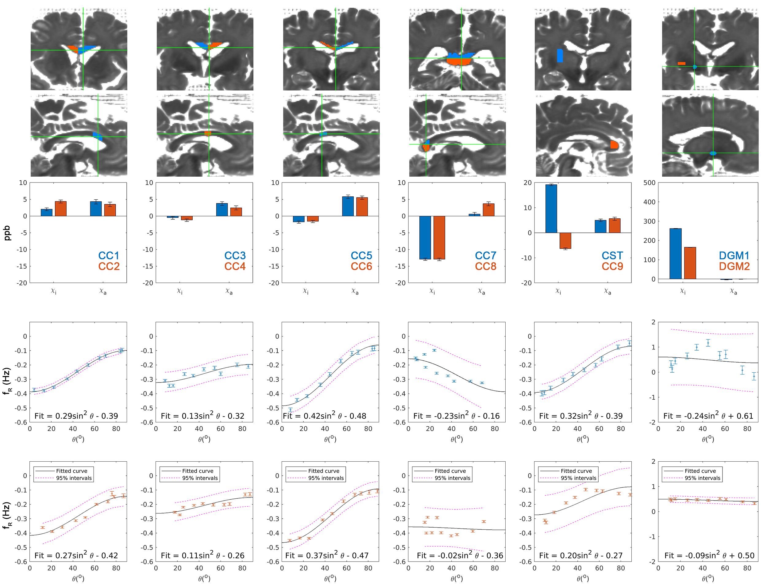
For the excised specimens immersed in agarose gel, quantification of isotropic ($$$\chi_{i}$$$) and anisotropic susceptibility ($$$\chi_{a}$$$) without non-susceptibility contributions as confounding factors was performed by fitting the field measured, $$$f_{N}$$$, surrounding the sample, $$$M_{out}$$$, considering that the tissue had a known fibre direction and constant properties throughout⁶:
$$\min_{\chi_{i},\chi_{a}}||M_{out}(f_{N}-\chi_{i}{\delta}f_{i_{sim}N}-\chi_{a}{\delta}f_{a_{sim}N})||[Eq.2]$$
where $$${\delta}f_{i_{sim}N}$$$ and $$${\delta}f_{a_{sim}N}$$$ are the simulated frequency perturbations per unit of isotropic and anisotropic magnetic susceptibility when the specimen was in orientation N. Subsequently, tissue non-susceptibility contributions to the phase can be measured as the residual field ($$$f_{R}$$$) inside the sample, $$$M_{in}$$$:
$$f_{R,N}=\overline{M_{in}(f_{N}-\chi_{i}{\delta}f_{i_{sim}N}-\chi_{a}{\delta}f_{a_{sim}N})}[Eq.3]$$
which was fitted with the following angular ($$$\theta$$$) dependence between fibre direction and B₀:
$$f_{R}=A\sin^2\theta+b[Eq.4]$$

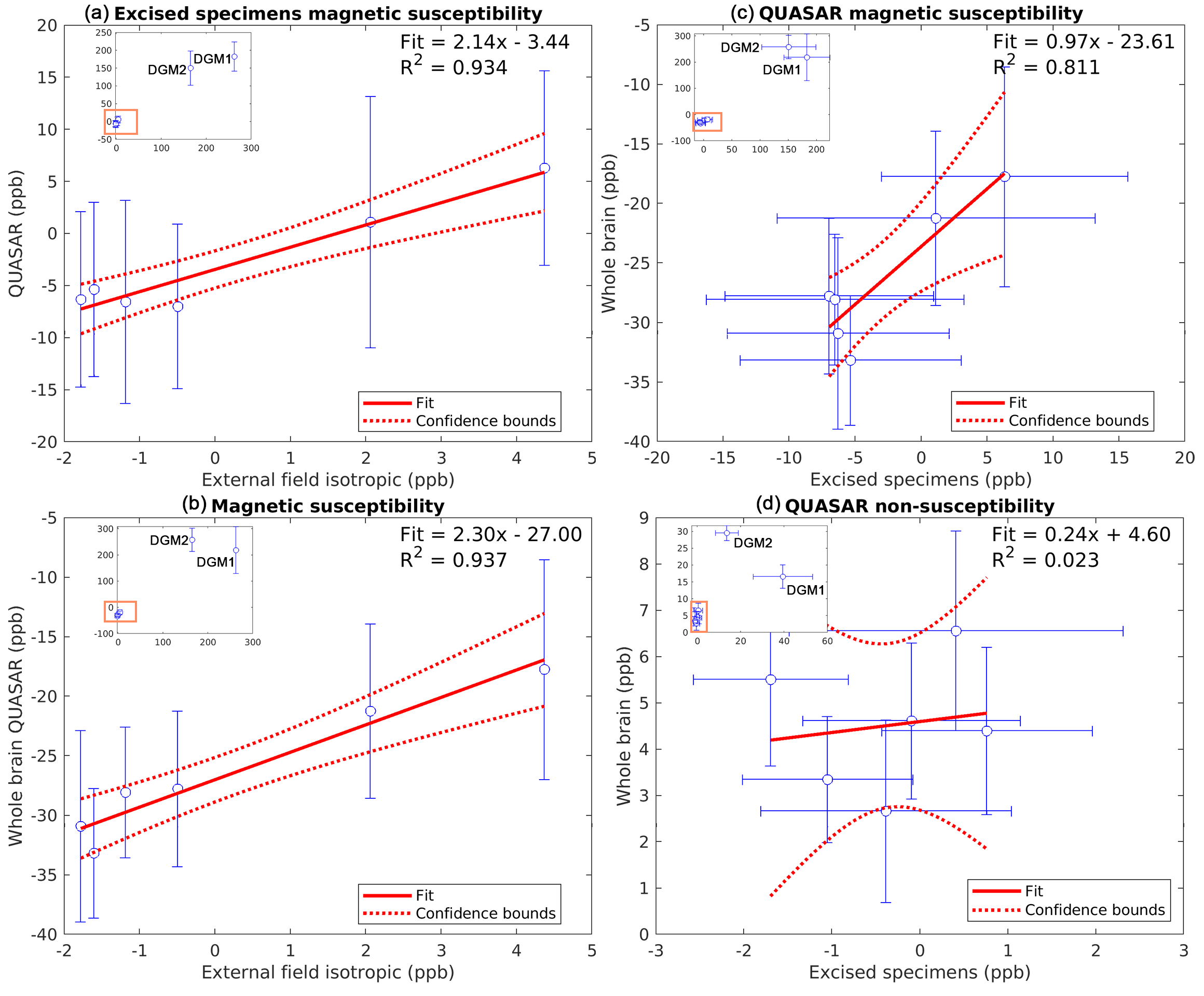
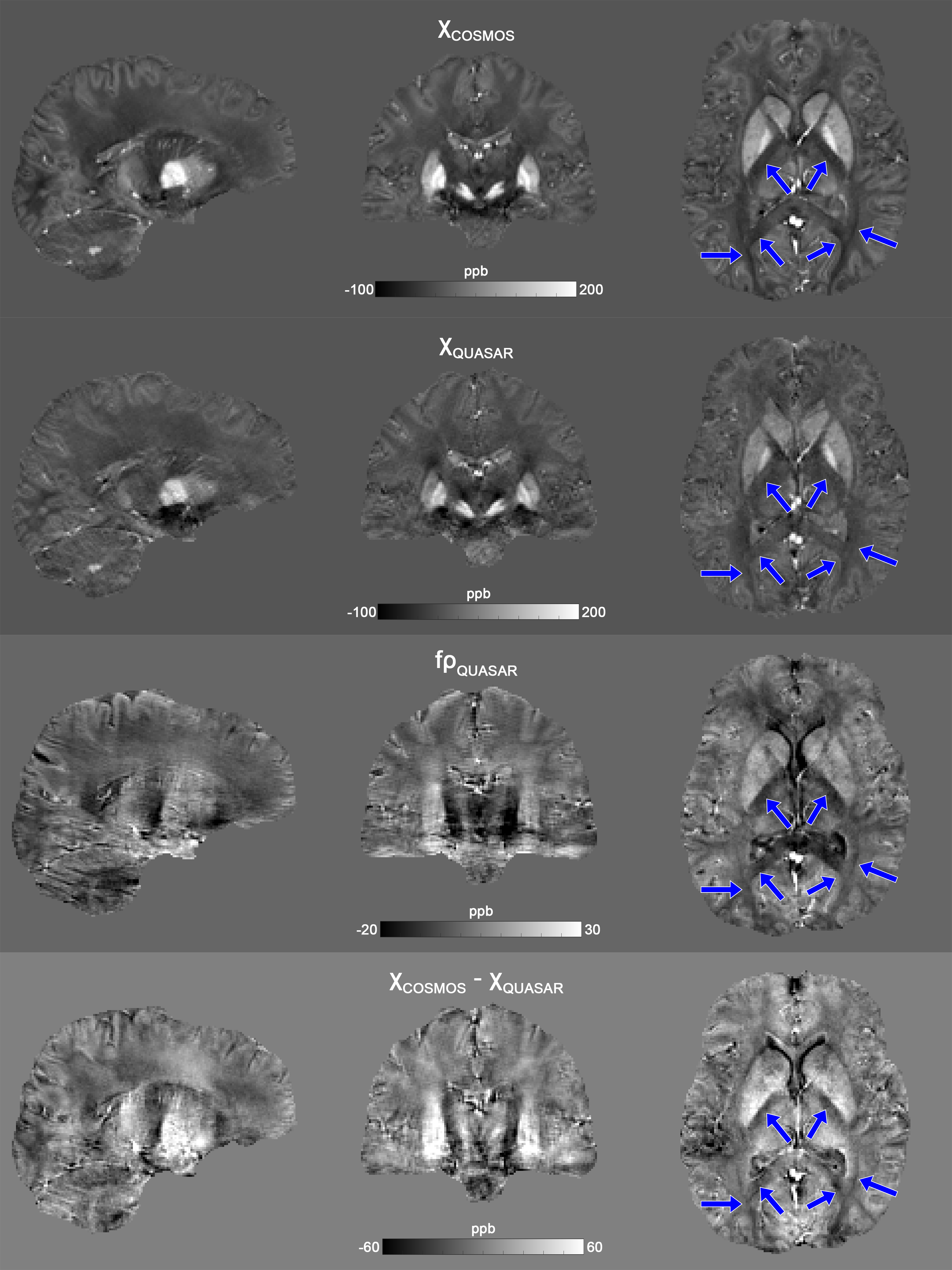
Linear regression analysis was conducted to compare magnetic susceptibility measured between various methods and between the two scanning sessions. Furthermore, an in-vivo dataset with 12 orientations to B₀ used for QSM Challenge 1²⁰ was processed with COSMOS²¹ and Eq.1 to understand the contrast we observed in our ex-vivo data.

Results and Discussion

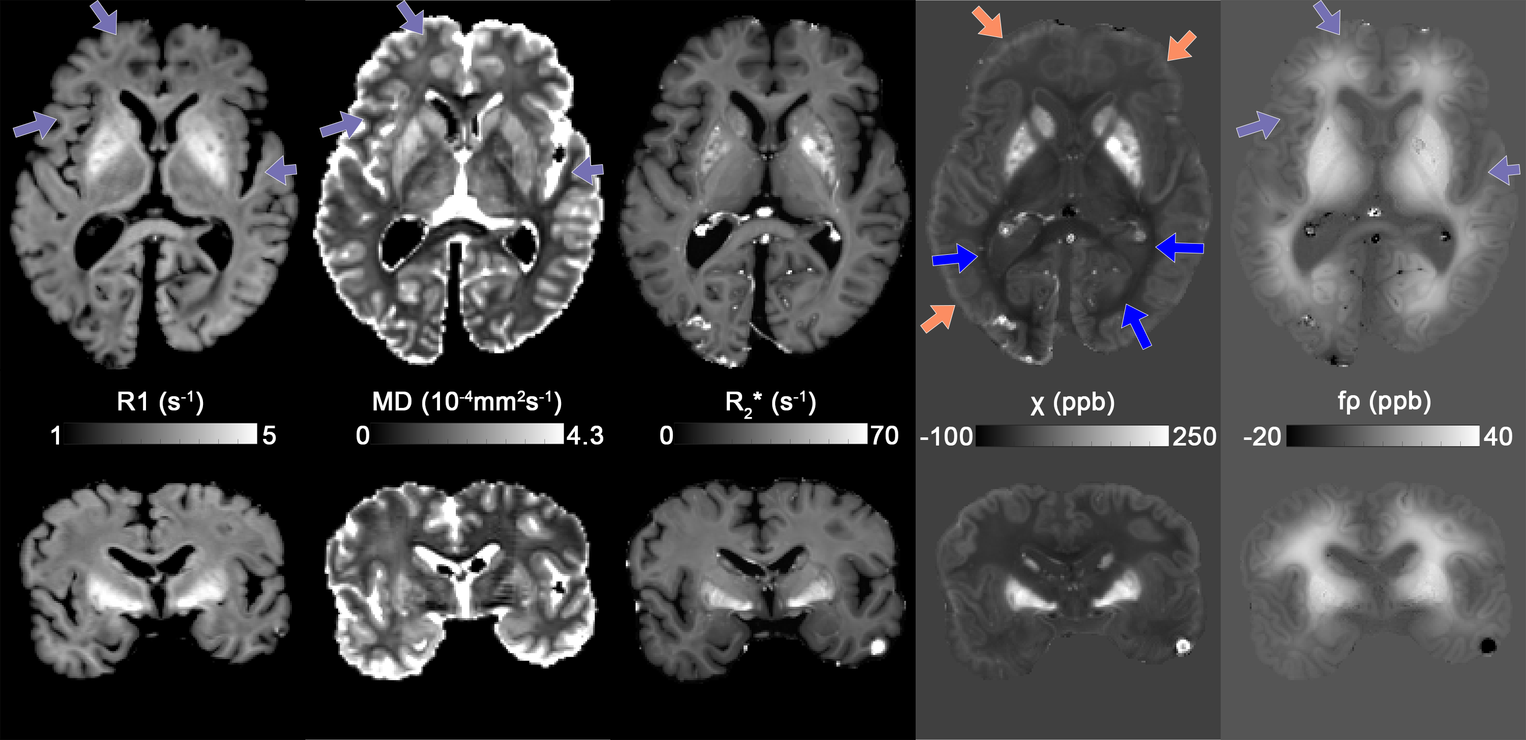
Fig.2 shows the R1, DTI mean diffusivity (MD), mean R₂*, QUASAR’s $$$\chi$$$ and QUASAR’s non-susceptibility source of the whole-brain specimen. R1 maps show WM and GM having comparable values while DGM has increased relaxation rates, suggesting iron as main contrast source. MD in WM is ~1.25x10^-4mm²/s which is significantly lower than in-vivo values (roughly 5-7x10^-4mm²/s).

All excised WM specimens had much lower $$$\chi_{i}$$$ measured using external fields (Fig.3) compared to fresh tissue ($$$\chi_{i}$$$=-81.5⁴/=-44¹²ppb), yet this parameter is also subject to the susceptibility of the embedding medium (in our case 1% agarose gel we estimated to have a susceptibility of -2.12ppb). The magnitude of $$$\chi_{a}$$$ is also lower but to a smaller degree ($$$\chi_{a}$$$=11.3⁴/=-45¹²/=-15¹²ppb). The $$$\sin^2{\theta}$$$ dependency of the samples is also weaker and have an opposite sign (-5.59Hz@7T⁴ corresponding to 18.8ppb), suggesting that the fixed tissue microstructure compartmental frequency is much weaker.

Linear regressions in Fig.4. shows strong correlations on WM magnetic susceptibility measurements within and across sessions, while the $$$\chi$$$ measured by QUASAR is about 2 times stronger than that estimated by the external field method. Both the in vivo non-susceptibility source maps (Fig.5) and the ex vivo maps (Fig.2) show cortical and deep GM that are brighter than the surrounding WM, and there are no significant differences among DGM. However, while the in vivo magnetic susceptibility map has reduced contrast within WM (blue arrows, Figs.2&5), these contrasts remain in the ex vivo result, indicating that the Lorentzian-sphere model can now account for the WM susceptibility differences because the compartmentalization effects are significantly reduced.

Conclusions

Formalin-fixed brain specimen has significantly different MR phase contrast from fresh tissue. Reduction of compartmentalisation was observed in the fixed tissue, and the non-susceptibility contributions are dominated by fixation artefact. Nevertheless, the non-susceptibility contributions share some similarities between in vivo and ex vivo imaging suggesting that significant exchange processes take place in iron-rich structures.

Acknowledgements

This work is part of the research programme with project number FOM-N-31/16PR1056/RadboudUniversity, which is financed by the Netherlands Organisation for Scientific Research (NWO).

References

1. Deistung, A., Schweser, F. & Reichenbach, J. R. Overview of quantitative susceptibility mapping. NMR in biomedicine30, (2016).

2. Wang, Y. & Liu, T. Quantitative susceptibility mapping (QSM): Decoding MRI data for a tissue magnetic biomarker. Magnetic Resonance in Medicine 73, 82–101 (2014).

3. Wharton, S. & Bowtell, R. Fiber orientation-dependent white matter contrast in gradient echo MRI. Proceedings of the National Academy of Sciences 109, 18559–18564 (2012).

4. Wharton, S. & Bowtell, R. Effects of white matter microstructure on phase and susceptibility maps. Magnetic resonance in medicine 73, 1258–1269 (2015).

5. Shmueli, K. et al. Magnetic susceptibility mapping of brain tissue in vivo using MRI phase data. Magnetic resonance in medicine 62, 1510–1522 (2009).

6. Zhong, K., Leupold, J., Elverfeldt, D. von & Speck, O. The molecular basis for gray and white matter contrast in phase imaging. Neuroimage 40, 1561–1566 (2008).

7. Luo, J., He, X., d’Avignon, D. A., Ackerman, J. J. H. & Yablonskiy, D. A. Protein-induced water 1H MR frequency shifts: Contributions from magnetic susceptibility and exchange effects. J Magn Reson 202, 102–108 (2010).

8. Li, W., Liu, C., Duong, T. Q., Zijl, P. C. M. van & Li, X. Susceptibility tensor imaging (STI) of the brain. NMR in biomedicine 30, e3540 (2017).

9. Yablonskiy, D. A. & Sukstanskii, A. L. Generalized Lorentzian Tensor Approach (GLTA) as a biophysical background for quantitative susceptibility mapping. Magnetic Resonance in Medicine 73, 757–764 (2015).

10. Shatil, A. S., Uddin, M. N., Matsuda, K. M. & Figley, C. R. Quantitative Ex Vivo MRI Changes due to Progressive Formalin Fixation in Whole Human Brain Specimens: Longitudinal Characterization of Diffusion, Relaxometry, and Myelin Water Fraction Measurements at 3T. Frontiers in medicine 5, 31 (2018).

11. Schmierer, K. et al. Quantitative magnetic resonance of postmortem multiple sclerosis brain before and after fixation. Magnetic resonance in medicine 59, 268–277 (2008).

12. Luo, J., He, X. & Yablonskiy, D. A. Magnetic susceptibility induced white matter MR signal frequency shifts--experimental comparison between Lorentzian sphere and generalized Lorentzian approaches. Magnetic resonance in medicine 71, 1251–1263 (2014).

13. Chan, K.-S. et al. 3D-Printed whole-brain holder for multiple orientation magnetic susceptibility measurements and precise dissection. in Proceedings 27. Annual Meeting International Society for Magnetic Resonance in Medicine vol. 27 5065 (http://archive.ismrm.org/2019/5065.html, 2019).

14. Avants, B. B. et al. A reproducible evaluation of ANTs similarity metric performance in brain image registration. Neuroimage 54, 2033–2044 (2011).

15. Karsa, A. & Shmueli, K. SEGUE: a Speedy rEgion-Growing algorithm for Unwrapping Estimated phase. IEEE Transactions on Medical Imaging 38, 1347–1357 (2018).

16. Robinson, S. D. et al. An illustrated comparison of processing methods for MR phase imaging and QSM: combining array coil signals and phase unwrapping. NMR in biomedicine 30, e3601 (2017).

17. Zhou, D., Liu, T., Spincemaille, P. & Wang, Y. Background field removal by solving the Laplacian boundary value problem. NMR in biomedicine 27, 312–319 (2014).

18. Chan, K.-S. & Marques, J. P. SEPIA - Susceptibility mapping pipeline tool for phase images. Neuroimage 117611 (2020) doi:10.1016/j.neuroimage.2020.117611.

19. Schweser, F. & Zivadinov, R. Quantitative susceptibility mapping (QSM) with an extended physical model for MRI frequency contrast in the brain: a proof‐of‐concept of quantitative susceptibility and residual (QUASAR) mapping. NMR in Biomedicine 31, e3999 (2018).

20. Milovic, C. et al. The 2016 QSM Challenge: Lessons learned and considerations for a future challenge design. Magnet Reson Med 84, 1624–1637 (2020).

21. Liu, T., Spincemaille, P., Rochefort, L. de, Kressler, B. & Wang, Y. Calculation of susceptibility through multiple orientation sampling (COSMOS): A method for conditioning the inverse problem from measured magnetic field map to susceptibility source image in MRI. Magnetic resonance in medicine 61, 196–204 (2009).

Figures

Fig. 1: An illustration of the experimental procedures. Before the experiment, the whole-brain specimen morphology was obtained from a pre-scan to create a custom-made holder to minimise tissue deformation and dislocation across scans. The specimen was then scanned with various sequences in the first session. After the session, the DWI data was processed with DTI model and the FA map was used to determine homogeneous WM samples. 12 brain samples (10WM + 2DGM) were excised and scanned in the second session.

Fig. 2: Transverse and coronal slices of quantitative R1, MD, R₂*, χ and f_ρ maps after fixation. Unlike in vivo, R1 maps show enhanced values in iron-rich DGM, similar to R₂* and χ, and greatly reduced GM & WM contrast and overall increased rates. MD in WM is much lower than typical in-vivo values (5-7x10^-4mm²/s). QUASAR χ shows fixation artefact at the brain surface (bright ring, orange arrows). The non-susceptibility source map contrast is dominated by fixation artefact (gradient change from brain surface toward the centre), which are also visible in R1 and MD maps (purple arrows).

Fig. 3: Top 2 rows show ROIs of excised samples. 3^rd row shows χ_iand χ_a of excised specimens measured by external field. Bottom 2 rows show residual field inside the sample fitted with Eq.4. WM at the genu and splenium of the corpus callosum (CC7-9) showed both the strongest diamagnetic isotropic susceptibility but very poorly described residual fields. The CST sample had residual DGM tissue in the corner of the sample, explaining the strong positive susceptibility compared to other WM. These 4 samples were excluded from the correlation analysis in Fig.4.

Fig. 4: Plots showing the correlation: (a) between QUASAR and external field measured χ from the 2^nd(excised samples) session, (b) and between the χ obtained in whole-brain QUASAR and the excised samples external field measurement, (c) QUASAR χ across both sessions and (d) non-susceptibility source across both sessions. Fitted intercepts in (b-c) are associated with the different medium used (1^st session: water; 2^ndsession:1% agarose). No relationship is observed on the non-susceptibility contributions measured by QUASAR.

Fig. 5: Magnetic susceptibility map (COSMOS & QUASAR) and non-susceptibility source map (QUASAR) from QSM Challenge 1 in vivo dataset. One notable difference between COSMOS and QUASAR is the contrasts within WM tissue vanished in the susceptibility map but these contrasts can be found in the non-susceptibility source maps (blue arrows). Comparing the in vivo non-susceptibility source maps to the ex vivo one shown in Fig.2, both show cortical and deep GM that are brighter than the WM locally, and there is no significant contrast among the basal ganglia.

Proc. Intl. Soc. Mag. Reson. Med. 29 (2021)

3970