3969
Validating DECOMPOSE QSM with temperature variant ex vivo brainstem imaging experiments1Department of Electrical Engineering and Computer Sciences, University of California, Berkeley, Berkeley, CA, United States, 2LIM44, Instituto e Departamento de Radiologia, Faculdade de Medicina, Universidade de Sao Paulo, Sao Paulo, Brazil, 3Helen Wills Neuroscience Institute, University of California, Berkeley, Berkeley, CA, United States
Synopsis
A model and corresponding solver for estimating sub-voxel paramagnetic and diamagnetic susceptibility components are validated based on the temperature dependence of magnetic susceptibility. Two pieces of brainstem sample were scanned under various temperature conditions to test the properties of the separated paramagnetic and diamagnetic components.
INTRODUCTION
Quantitative susceptibility mapping (QSM) is sensitive to tissue’s molecular composition1. QSM has been applied in multiple clinical and research settings, from developing diagnostic biomarker of dementia 2,3,4,5,6 to understanding cerebral structures7,8 and to monitoring disease treatment9. However, colocalization of species with opposing susceptibility confounds the quantification of magnetic susceptibility. For instance, colocalization of iron with Amyloid beta in Alzheimer’s disease patients is known and QSM has been applied to study such.6,10–12 A couple of models have been proposed to decompose QSM.13,14 Among those, qualitative histological staining is the most common in vivo validation. Here, we use temperature-dependent GRE data to validate the separation of a newly proposed DECOMPOSE QSM.THEORY
Paramagnetism and diamagnetism are the two most commonly found magnetic properties of biologic tissues. Following Curie’s Law, at a certain range of temperature and field strength, paramagnetic susceptibility is approximately inversely proportional to temperature, $$\begin{align} \chi (T\rightarrow \infty) = \frac{C}{T} \end{align} \tag{1}$$ where C is the material’s specific Curie constant. We propose to use this relationship to validating algorithms for decomposing QSM sources. Specifically, the paramagnetic component should be temperature dependent while the diamagnetic component should remain stable across temperature changes. There has been study shown that such an effect is visible through QSM15.'The model we are validating here is the DiamagnEtic-COMponent-and-Paramagnetic-cOmponent-SEparation (DECOMPOSE) QSM based on a three-pool signal model as$$\begin{align}S(t;C_+,C_-,C_0,\chi_+,\chi_-,R^*_{2,0})=&C_+e^{-(a\chi_++R^*_{2,0}+i\frac{2}{3}\chi_+\gamma B_0)t}\\&+C_-e^{-(-a\chi_-+R^*_{2,0}+i\frac{2}{3}\chi_-\gamma B_0)t}\\&+ C_0e^{-R^*_{2,0}t}\end{align}\tag{2}$$
where paramagnetic, diamagnetic and neutral-susceptibility components contribute one term each of complex exponential to the total signal of a voxel. The estimated parameters are used to form Paramagnetic Component Susceptibility (PCS) and Diamagnetic Component Susceptibility (DCS) defined as below,
$$\text{PCS (or DCS)}=\frac{\sum_t\measuredangle(C_{+or-}e^{-(a|\chi_{+or-}|+R^*_{2,0}+i\frac{2}{3}\chi_{+or-}\gamma B_0)t}+(C_0+C_{-,or +})e^{-R^*_{2,0}t})}{\frac{2}{3}\gamma B_0\sum t}\tag{3}$$.
METHODS
Two human brainstems were fixed in a non-buffered 4%-formalin for over 12 months, washed out in distilled water and placed into a proton-free fluid (Fomblin) prior to MRI scanning. Fomblin produces no MRI signal and has a similar susceptibility to tissue16. Sample tube was heated up using water bath for 3 hours at 40oC before the acquisition on 7T Magnetom (SIEMENS, Erlangen, Germany) using an in-house built solenoid.QSM acquisition was repeated sequentially while the brainstem was cooling down naturally until reaching thermal equilibrium (20°C). A 3D muilti-echo FLASH GRE was used with the following parameters:FOV=120mm, voxelsize=0.25x0.25x0.4mm3. Two sets of data were acquired: one with five echoes of TE1/deltaTE/TE5 = 4/3/16ms, and the other with 16 echoes of TE1/deltaTE/TE16=4/3/49ms. Due to low SNR of later echoes, only the first 12 echoes were adopted for further analysis.
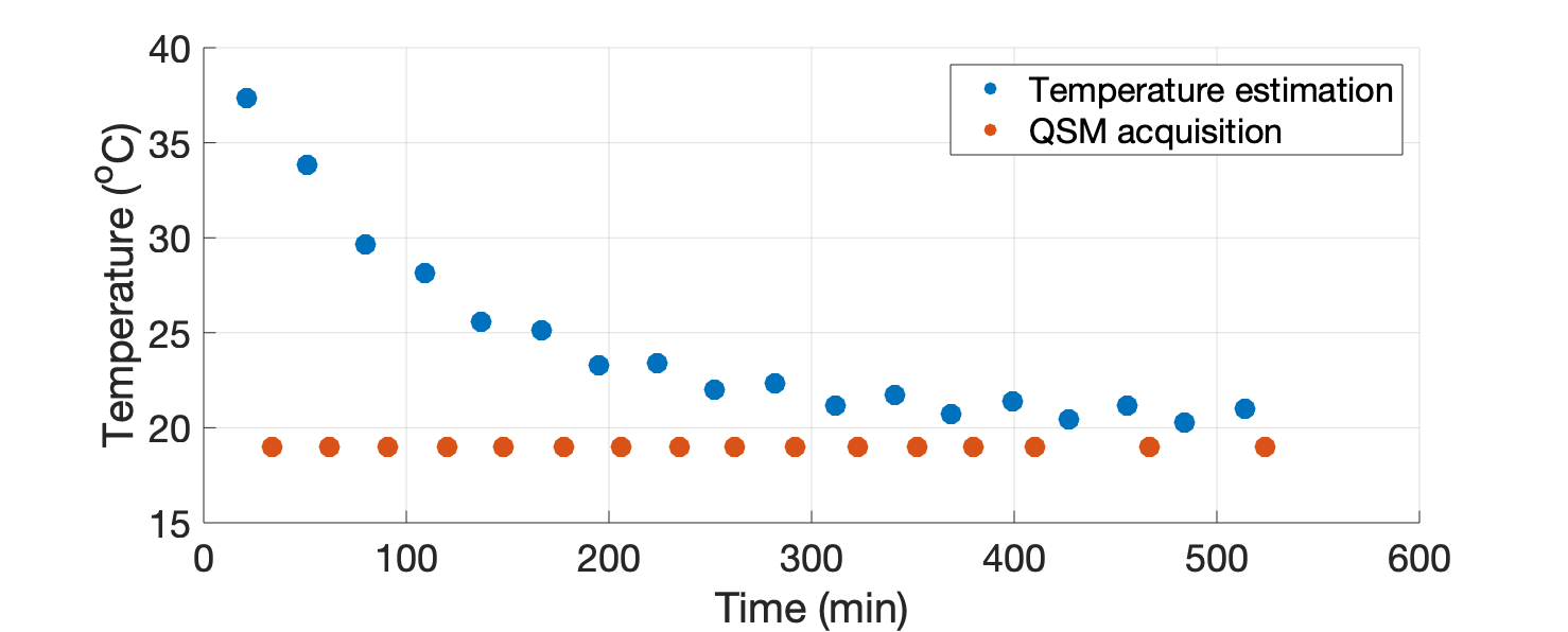
Before every GRE acquisition, a single-shot water unsuppressed spectrum was acquired with semiLASER sequence, with TE/TM/TR=7/26/9000 ms, voxelsize = 30x20x20 mm3 to estimate temperature through chemical shift from the spectrum.
Phase is unwrapped by Laplacian-based method17,18 followed by V-SHARP19 background removal. Lastly, QSM of each echo was computed using STAR-QSM20 in STI Suite21. The resulting QSM maps are re-referenced to the region where $$$R_2^*$$$ value has lower than 4 Hz2 variance over time.
RESULTS
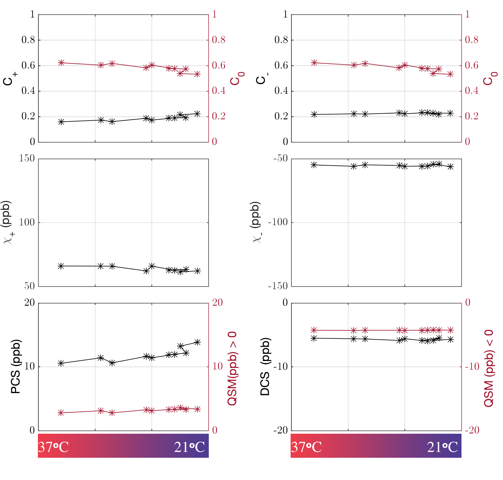
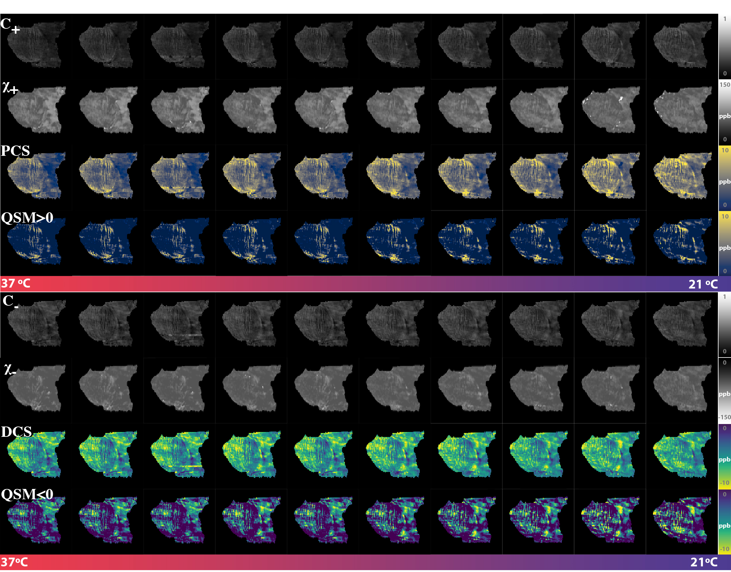
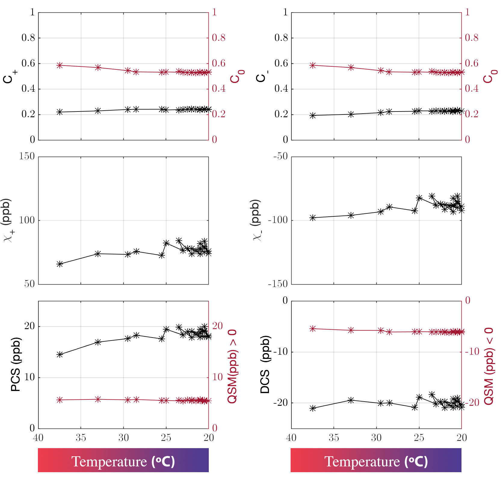
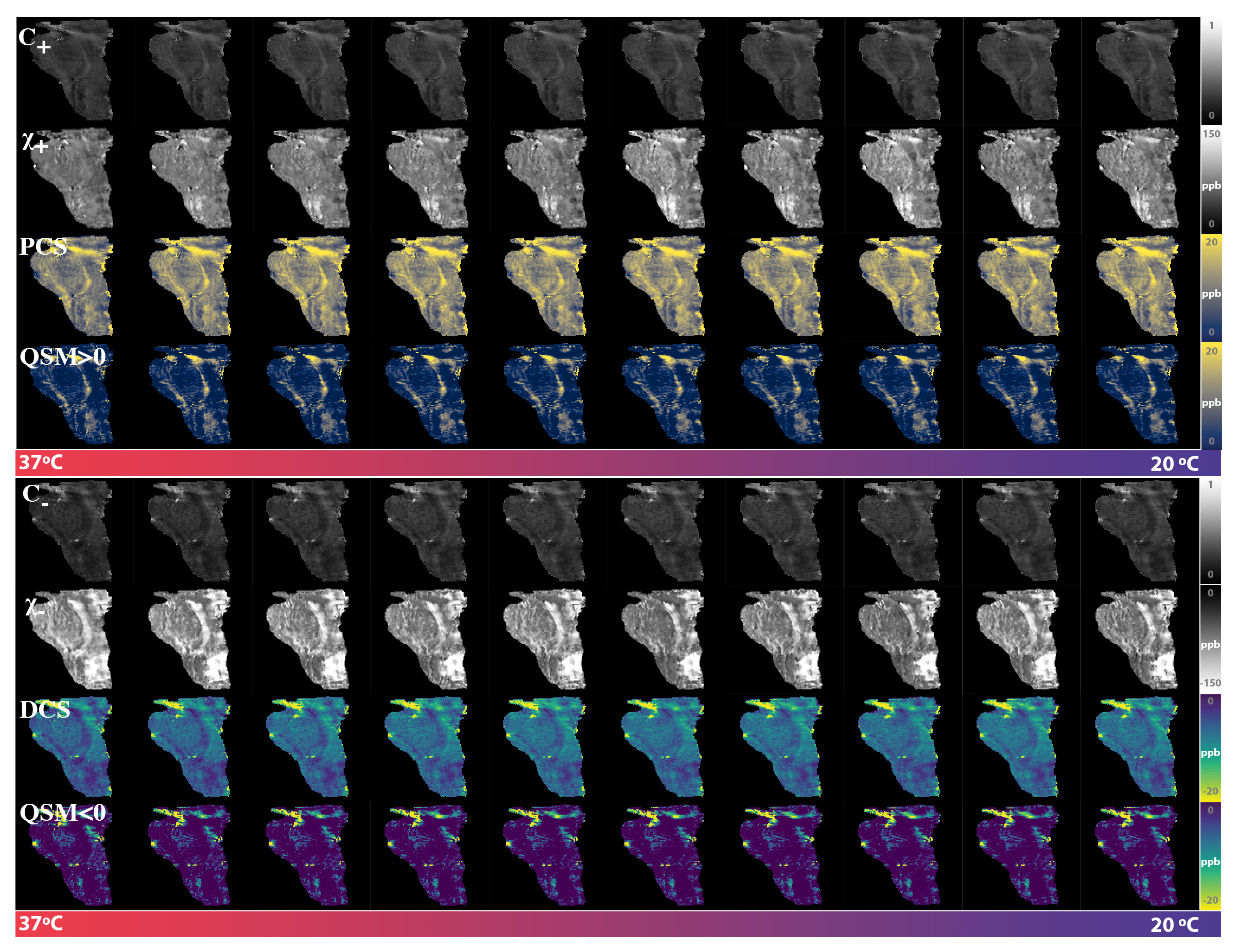
Figure 1 shows a plot of the indirect measurement of temperature through analyzing water proton chemical shift as a function of time. The DECOMPOSE results of each set of data are presented as line graphs and corresponding parameter maps. The resulting paramagnetic component susceptibility (PCS) (Figure 2,4) showed more visible increases as the temperature decreases. The diamagnetic component susceptibility (DCS) showed minimal changes across the scans. Detailed parameter maps of one sagittal slice are shown in Figure 3,5. With either 5 or 12 echoes, the resulting PCS visibly increase as the temperature decreases. Further, it appears that decomposing with the 12-echo data results in more temperature-stable DCS maps.DISCUSSION
The method we are validating is based on multi-echo GRE data. Generally, more echoes are beneficial since the model relies on the temporal behavior of the signal progression. Here we show that, in practice, with as minimal as 5 echoes, the algorithm is able to separate para-/dia-magnetism with reasonable results.One big challenge in performing the analysis was the lack of an absolute reference for QSM. As temperature changes, the absolute bulk susceptibility of the whole sample changes. Larmor frequency shift and phase pre-processing employed in QSM reconstruction methods remove the zero and first-order information of the phase, which leads to the QSM being referenced to the mean of the whole sample with STAR-QSM. As the temperature decreases, total bulk susceptibility increases with paramagnetic susceptibility's increase, which will then lead to an apparent decrease of the diamagnetic part whereas the physical diamagnetic susceptibility ought to remain stable with temperature changes. To address this, we used regions with minimum $$$R_2^*$$$ temporal variation as QSM reference. Even so, changes in DCS may still be observed but less dramatic than that of PCS.
The volume fractions ($$$C_{+,-,0}$$$) also showed a slight temperature dependance. We estimated that the thermal expansion resulting from a 20-degree-Celsius range will lead to approximately 0.5% of volume change if extracellular fluid is considered to have volume thermal expansion coefficient close to water22 and up to 1.5% if proteins/lipids and other biomolecules are considered23. This is comparable to what we have observed. Nonetheless, the estimation of parameters may be corrupted by noise and QSM inaccuracies, thus caution is warranted in interpreting the results.
Acknowledgements
No acknowledgement found.References
(1) Liu, C.; Wei, H.; Gong, N.-J.; Cronin, M.; Dibb, R.; Decker, K. Quantitative Susceptibility Mapping: Contrast Mechanisms and Clinical Applications. Tomography 2015, 1 (1), 3–17. https://doi.org/10.18383/j.tom.2015.00136.
(2) Guan, X.; Huang, P.; Zeng, Q.; Liu, C.; Wei, H.; Xuan, M.; Gu, Q.; Xu, X.; Wang, N.; Yu, X.; Luo, X.; Zhang, M. Quantitative Susceptibility Mapping as a Biomarker for Evaluating White Matter Alterations in Parkinson’s Disease. Brain Imaging Behav 2019, 13 (1), 220–231. https://doi.org/10.1007/s11682-018-9842-z.
(3) He, N.; Ling, H.; Ding, B.; Huang, J.; Zhang, Y.; Zhang, Z.; Liu, C.; Chen, K.; Yan, F. Region-Specific Disturbed Iron Distribution in Early Idiopathic Parkinson’s Disease Measured by Quantitative Susceptibility Mapping. Human Brain Mapping 2015, 36 (11), 4407–4420. https://doi.org/10.1002/hbm.22928.
(4) Wisnieff, C.; Ramanan, S.; Olesik, J.; Gauthier, S.; Wang, Y.; Pitt, D. Quantitative Susceptibility Mapping (QSM) of White Matter Multiple Sclerosis Lesions: Interpreting Positive Susceptibility and the Presence of Iron. Magnetic Resonance in Medicine 2015, 74 (2), 564–570. https://doi.org/10.1002/mrm.25420.
(5) Zhang, Y.; Gauthier, S. A.; Gupta, A.; Comunale, J.; Chiang, G. C.-Y.; Zhou, D.; Chen, W.; Giambrone, A. E.; Zhu, W.; Wang, Y. Longitudinal Change in Magnetic Susceptibility of New Enhanced Multiple Sclerosis (MS) Lesions Measured on Serial Quantitative Susceptibility Mapping (QSM). Journal of Magnetic Resonance Imaging 2016, 44 (2), 426–432. https://doi.org/10.1002/jmri.25144.
(6) Gong, N.-J.; Dibb, R.; Bulk, M.; van der Weerd, L.; Liu, C. Imaging Beta Amyloid Aggregation and Iron Accumulation in Alzheimer’s Disease Using Quantitative Susceptibility Mapping MRI. NeuroImage 2019, 191, 176–185. https://doi.org/10.1016/j.neuroimage.2019.02.019.
(7) Wei, H.; Xie, L.; Dibb, R.; Li, W.; Decker, K.; Zhang, Y.; Johnson, G. A.; Liu, C. Imaging Whole-Brain Cytoarchitecture of Mouse with MRI-Based Quantitative Susceptibility Mapping. NeuroImage 2016, 137, 107–115. https://doi.org/10.1016/j.neuroimage.2016.05.033.
(8) Zhang, Y.; Wei, H.; Cronin, M. J.; He, N.; Yan, F.; Liu, C. Longitudinal Atlas for Normative Human Brain Development and Aging over the Lifespan Using Quantitative Susceptibility Mapping. NeuroImage 2018, 171, 176–189. https://doi.org/10.1016/j.neuroimage.2018.01.008.
(9) Zhang, Y.; Wei, H.; Sun, Y.; Cronin, M. J.; He, N.; Xu, J.; Zhou, Y.; Liu, C. Quantitative Susceptibility Mapping (QSM) As a Means to Monitor Cerebral Hematoma Treatment. J Magn Reson Imaging 2018, 48 (4), 907–915. https://doi.org/10.1002/jmri.25957.
(10) Ayton, S.; Wang, Y.; Diouf, I.; Schneider, J. A.; Brockman, J.; Morris, M. C.; Bush, A. I. Brain Iron Is Associated with Accelerated Cognitive Decline in People with Alzheimer Pathology. Molecular Psychiatry 2020, 25
(11), 2932–2941. https://doi.org/10.1038/s41380-019-0375-7.(11) Duce, J. A.; Tsatsanis, A.; Cater, M. A.; James, S. A.; Robb, E.; Wikhe, K.; Leong, S. L.; Perez, K.; Johanssen, T.; Greenough, M. A.; Cho, H.-H.; Galatis, D.; Moir, R. D.; Masters, C. L.; McLean, C.; Tanzi, R. E.; Cappai, R.; Barnham, K. J.; Ciccotosto, G. D.; Rogers, J. T.; Bush, A. I. Iron-Export Ferroxidase Activity of β-Amyloid Precursor Protein Is Inhibited by Zinc in Alzheimer’s Disease. Cell 2010, 142 (6), 857–867. https://doi.org/10.1016/j.cell.2010.08.014.
(12) Telling, N. D.; Everett, J.; Collingwood, J. F.; Dobson, J.; van der Laan, G.; Gallagher, J. J.; Wang, J.; Hitchcock, A. P. Iron Biochemistry Is Correlated with Amyloid Plaque Morphology in an Established Mouse Model of Alzheimer’s Disease. Cell Chemical Biology 2017, 24 (10), 1205-1215.e3. https://doi.org/10.1016/j.chembiol.2017.07.014.
(13) Schweser, F.; Deistung, A.; Lehr, B.; Sommer, K.; Reichenbach, J. SEMI-TWInS: Simultaneous Extraction of Myelin and Iron Using a T2*-Weighted Imaging Sequence. In Proceedings of the 19th Meeting of the International Society for Magnetic Resonance in Medicine; 2011; p 120.
(14) Lee, J.; Nam, Y.; Choi, J. Y.; Shin, H.; Hwang, T.; Lee, J. Separating Positive and Negative Susceptibility Sources in QSM. ISMRM, HONOLULU, HI, USA, MRM.[Google Scholar] 2017.
(15) Birkl, C.; Langkammer, C.; Krenn, H.; Goessler, W.; Ernst, C.; Haybaeck, J.; Stollberger, R.; Fazekas, F.; Ropele, S. Iron Mapping Using the Temperature Dependency of the Magnetic Susceptibility. Magnetic Resonance in Medicine2015, 73 (3), 1282–1288. https://doi.org/10.1002/mrm.25236.
(16) Shatil, A. S.; Matsuda, K. M.; Figley, C. R. A Method for Whole Brain Ex Vivo Magnetic Resonance Imaging with Minimal Susceptibility Artifacts. Front. Neurol. 2016, 7. https://doi.org/10.3389/fneur.2016.00208.
(17) Schofield, M. A.; Zhu, Y. Fast Phase Unwrapping Algorithm for Interferometric Applications. Opt Lett 2003, 28(14), 1194–1196. https://doi.org/10.1364/ol.28.001194.
(18) Li, W.; Wu, B.; Liu, C. Quantitative Susceptibility Mapping of Human Brain Reflects Spatial Variation in Tissue Composition. Neuroimage 2011, 55 (4), 1645–1656. https://doi.org/10.1016/j.neuroimage.2010.11.088.
(19) Wu, B.; Li, W.; Guidon, A.; Liu, C. Whole Brain Susceptibility Mapping Using Compressed Sensing. Magnetic Resonance in Medicine 2012, 67 (1), 137–147. https://doi.org/10.1002/mrm.23000.
(20) Wei, H.; Dibb, R.; Zhou, Y.; Sun, Y.; Xu, J.; Wang, N.; Liu, C. Streaking Artifact Reduction for Quantitative Susceptibility Mapping of Sources with Large Dynamic Range. NMR Biomed 2015, 28 (10), 1294–1303. https://doi.org/10.1002/nbm.3383.(21) STI Suite V3.0 https://people.eecs.berkeley.edu/~chunlei.liu/software.html.
(22) Thermal Expansion. Wikipedia; 2020.
(23) Rabin, Y.; Plitz, J. Thermal Expansion of Blood Vessels and Muscle Specimens Permeated with DMSO, DP6, and VS55 at Cryogenic Temperatures. Ann Biomed Eng 2005, 33 (9), 1213–1228. https://doi.org/10.1007/s10439-005-5364-0.
Figures