Introduction

$$$\,\,\,\,\,\,$$$Recently, the magnetic susceptibility source separation method or 𝜒-separation was proposed to estimate the individual concentration of positive ($$$\chi_{pos}$$$) and negative susceptibility ($$$\chi_{neg}$$$)¹. This method potentially enables to quantify two dominant susceptibility contributors in the brain, iron and myelin. In this work, we validate the 𝜒-separation model using Monte-Carlo simulation and test its capability to image iron and myelin by applying the method to ex-vivo and in-vivo brains and comparing the results with iron and myelin histology.

Methods

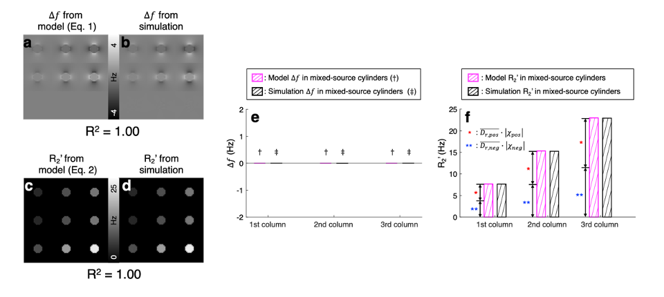
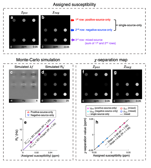
$$$\,\,\,\,\,\,$$$[𝜒-separation model] The frequency shift from the positive and negative susceptibility sources is modeled as follows²:$$\Delta{f}=D_{f}\,(r)\,{*}\,(\,{\chi_{pos}}\,+\,{\chi_{neg}}\,)\,\,\,\,\,\,\,[Eq. 1]$$where $$$D_{f}$$$ denotes the magnetic dipole kernel. For the reversible transverse relaxation rate (i.e., R2'=R2*-R2), the susceptibility sources can be modeled as follows^1,3:$$R_2'=D_{pos}\cdot{\lvert}{\chi_{pos}}{\rvert}+D_{neg}\cdot{\lvert}{\chi_{neg}}{\rvert}\,\,\,\,\,\,\,[Eq. 2]$$where $$$D_{pos}$$$ and $$$D_{neg}$$$ are the proportionality constants between R2' vs. positive and negative susceptibility, respectively. By exploiting both Eq. 1 and 2, the individual positive and negative susceptibility can be separately estimated⁴.
$$$\,\,\,\,\,\,$$$[Monte-Carlo simulation] Diffusion simulation with spherical susceptibility sources randomly distributed inside virtual cylinder was performed using the following parameters: matrix size=26 × 26 × 32, cylinder radius=4 voxels, diffusion coefficient=1 μm²/ms, source radius=1 μm, source susceptibility=520 ppm⁵, time step=100 μm, number of spins per voxel=400,000, and field strength=3T. Nine simulations were conducted with different susceptibility concentrations (12.5:12.5:37.5 ppb) and susceptibility compositions (positive-source-only, negative-source-only, and mixed-source) as visualized in Fig. 2a-b. $$$D_{pos}$$$ and $$$D_{neg}$$$ were estimated as the slope of R2' values with respect to absolute QSM values in the positive-source-only and negative-source-only cylinders, respectively.
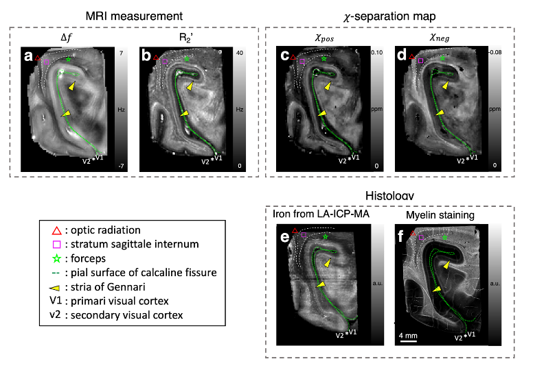
$$$\,\,\,\,\,\,$$$[Ex-vivo experiment] A paraformaldehyde-fixed ex-vivo brain specimen containing primary visual cortex was scanned at 7T. For R2* and frequency shift, multi-echo gradient-echo data were acquired using the following parameters: resolution=0.3 × 0.3 × 0.5 mm³, TR=300 ms, TE=3.9:6.5:39.8 ms, flip angle=45°, two averages, and scan time=4.8 h. For R2, multi-echo spin-echo data were collected using the following protocols: resolution=0.3 × 0.3 × 0.5 mm³, TR=450 ms, TE=14:14:70 ms, three averages, and scan time=10.6 h. The paraffin-embedded sections of the specimen were utilized for myelin staining using Luxol fast blue (LFB) and iron quantification using laser ablation-inductively coupled plasma-mass spectrometry (LA-ICP-MS). The proportionality constants of in-vivo volunteers (see next section) were utilized after scaling for field strength.
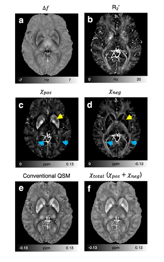
$$$\,\,\,\,\,\,$$$[In-vivo experiment] Six volunteers were scanned at 3T MRI. Multi-echo gradient-echo data were acquired using the following protocols: resolution=1 × 1 × 2 mm³, TR=64 ms, TE=2.9:4.6:25.9 ms, flip angle=22°, and scan time=7 min. 2D multi-echo spin-echo data were collected using the following parameters: resolution=1 × 1 mm², slice thickness=2 mm, TR=3860 ms, TE=15:15:90 ms, and scan time=12.4 min. To consider source characteristics of the human brain different with the simulation (see Discussion), $$$D_{pos}$$$ was estimated in five deep gray matter regions (putamen, globus pallidus, caudate nucleus, red nucleus, and substantia nigra), which primarily have positive susceptibility. For $$$D_{neg}$$$, the same value as $$$D_{pos}$$$ was used.

Results

$$$\,\,\,\,\,\,$$$To validate susceptibility models of 𝜒-separation (i.e., Eqs. 1 and 2), the frequency shift and R2' maps from the simulation are compared to those generated by Eqs. 1 and 2 (Fig. 1). The simulated frequency shift and R2' maps demonstrate strong correlations with the model predictions (voxel-wise linear regression: R²>0.99). The quantitative comparison results also support the model validity (Fig. 1e-f).
$$$\,\,\,\,\,\,$$$When the positive and negative susceptibility values from 𝜒-separation are compared to the assigned values in single-source-only cylinders (i.e., first-row and second-row cylinders) and mixed-source cylinders (i.e., third-row cylinders), strong correlations are observed (Fig. 2; linear regression slope=0.99 and R²=1.00), demonstrating successful separation of the sources.
$$$\,\,\,\,\,\,$$$For the ex-vivo specimen, the positive and negative susceptibility maps reveal great similarities with histologically-obtained iron and myelin images (Fig. 3), despite the complex microstructural environment of the brain. In the middle layer of the cortex, distinct hyperintensities are observed in both positive and negative susceptibility maps, revealing stria of Gennari, which is known to have higher iron and myelin concentration than other layers⁶. The same characteristics are also captured in iron and myelin images (Fig. 3e-f). Additionally, the 𝜒-separation maps delineate anatomical structures of white matter (optic radiation, stratum sagittale internum, and forceps), which are observable in the histological images.
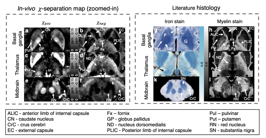
$$$\,\,\,\,\,\,$$$The in-vivo 𝜒-separation maps render well-known characteristics of iron and myelin distribution, suggesting the potential of the method for in-vivo iron and myelin mapping (Fig. 4). When the maps are zoomed-in and compared to histological images from literature^7–9, the subtle details of iron and myelin are delineated in the positive and negative susceptibility maps, respectively (Fig. 5).

Discussion

$$$\,\,\,\,\,\,$$$The proportionality constants ($$$D_{pos}$$$ and $$$D_{neg}$$$ ) can be influenced by the characteristics of susceptibility sources (size, geometry, and characteristic frequency of the sources)^10–12. Despite the difference in the proportionality constants (simulation: 321 Hz/ppm vs. in-vivo: 137 Hz/ppm), the successful delineation of histological iron and myelin distributions in both ex-vivo and in-vivo brains may indicate that the in-vivo proportionality constant may reflect in-vivo brain characteristics.

Concusion

$$$\,\,\,\,\,\,$$$The 𝜒-separation successfully reconstruct the positive and negative susceptibility in the Monte-Carlo simulation and, furthermore, delineate the exquisite details of iron and myelin distributions not only in the ex-vivo brain specimen but also in the in-vivo brain, suggesting the feasibility of iron and myelin mapping using 𝜒-separation.

Acknowledgements

This work was supported by the National ResearchFoundation of Korea (NRF) grant funded by the Korea government (MSIT) (No. NRF-2018R1A2B3008445)