Introduction

Features such as brain-calcification¹ demyelination² and iron-dyshomeostasis³ are associated with various neurodegenerative diseases, yet their noninvasive characterisation is a formidable challenge. MRI-driven mapping of magnetic tissue properties, including the local Larmor frequency, is promising for providing insights into such features, but both susceptibility and microstructure play important roles in the signal formation^4,5,6,7, which hampers accurate measurements without impractical sample rotations. The aim of the study is to bypass sample rotations by combining diffusion MRI and susceptibility-based MRI, which enables utilising information from the fiber orientation distribution function (fODF) as determined by diffusion imaging⁹. This, in turn, enables the estimation of the Larmor frequency and thereby a new means for characterising magnetic properties without sample rotation.

Theory

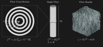
We model white matter as a medium of long hollow impermeable cylindrical inclusions. The inclusions are made of concentric shells, representing myelin, with an isotropic susceptibility $$$\chi$$$ relative to the surrounding MRI-visible fluid (figure 1), as a first approximation. The surroundings correspond to intra-axonal, extra-axonal and interstitial bi-layers. The inclusions occupy $$$\zeta{V}$$$ of the total volume $$$V,$$$ and are placed according to the indicator function $$$\nu(\mathbf{r})$$$. Placed in a static field $$$(B_0)_\alpha=B_0{{n}}_{\alpha}^{{B}},$$$ a shift in the local Larmor frequency $$\Omega(r)=\gamma B_{0}\chi{n}_{\alpha}^{B}{n}_{\beta}^{B}\int_{V}d\mathbf{r}^{\prime}\mathcal{Y}_{\alpha\beta}\left(\mathbf{r}^{\prime}-\mathbf{r}\right)\nu\left(\mathbf{r}^{\prime}\right)\qquad\qquad(1)$$ is induced in the fluid, where $$$\mathcal{Y}_{\alpha\beta}$$$ is the Lorentz-corrected elementary dipole-field⁸. The normalized FID signal $$$S_k(t)$$$ from the MRI-visible fluid within an Isotropic voxel $$$V_k\in{V}$$$ is given by the ensemble average $$$\langle\cdot\rangle$$$ $$S_{k}(t)=e^{-R_{2}^{mol}t}\left\langle{e}^{-i\varphi_{k}(t)}\right\rangle,\qquad\varphi_{k}(t)=\int_{0}^{t}dt^{\prime} \Omega_{\mathrm{k}}\left(\mathbf{r}\left(t^{\prime}\right)\right).\qquad\qquad(2)$$ Here, $$$R_{2}^{mol}$$$ accounts for the irreversible molecular relaxation¹⁰. The first cumulant $$$\langle\Omega\rangle_k$$$ can be found from the signal derivative $$-Im\left\{\left.\frac{d}{dt}S_{k}(t)\right|_{t\rightarrow{0}}\right\}=\langle\Omega\rangle_{k},\qquad\qquad(3)$$ and $$$\langle\Omega\rangle_k$$$ may be obtained as $$\langle\Omega\rangle_{k}=\gamma{B}_{0}\chi{n}_{\alpha}^{B}{n}_{\beta}^{B}\frac{1}{\left(1-\zeta_{k}\right)V_{k}}\int_{V_{k}}d\boldsymbol{r}(1-v(\boldsymbol{r}))\int_{V}d\boldsymbol{r}^{\prime}\mathcal{Y}_{\alpha\beta}\left(\boldsymbol{r}^{\prime}-\boldsymbol{r}\right)v\left(\boldsymbol{r}^{\prime}\right).\qquad\qquad(4)$$ $$$\langle\Omega\rangle_k$$$ is described by the average static field within $$$V_k$$$, averaged over both intra-axonal, extra-axonal and interstitial bi-layers. Within the mesoscopic cavity approach^4,5,6,8, $$$\langle\Omega\rangle_k$$$ is divided into mesoscopic and macroscopic contributions, $$$\langle\Omega\rangle_k=\langle\Omega\rangle^{Meso}_k+\langle\Omega\rangle^{Macro}_k$$$, with $$\begin{array}{l}\langle\Omega\rangle_{k}^{Meso}=\gamma{B}_{0}\chi{n}_{\alpha}^{B}{n}_{\beta}^{B}\frac{1}{\left(1-\zeta_{k}\right)V_{k}}\int_{V_{k}}d\boldsymbol{r}(1-\nu(\boldsymbol{r}))\int_{\boldsymbol{r}^{\prime}\in\mathcal{M}(\boldsymbol{r})}d\boldsymbol{r}^{\prime}\mathcal{Y}_{\alpha\beta}\left(\boldsymbol{r}^{\prime}-\boldsymbol{r}\right)\nu\left(\boldsymbol{r}^{\prime}\right)\\\langle\Omega\rangle_{k}^{Macro}=\gamma{B}_{0}\chi{n}_{\alpha}^{B}{n}_{\beta}^{B}\frac{1}{\left(1-\zeta_{k}\right)V_{k}}\int_{V_{k}}d\boldsymbol{r}(1-\nu(\boldsymbol{r}))\int_{\boldsymbol{r}^{\prime}\notin\mathcal{M}(\boldsymbol{r})}d\boldsymbol{r}^{\prime}\mathcal{Y}_{\alpha\beta}\left(\boldsymbol{r}^{\prime}-\boldsymbol{r}\right)\nu\left(\boldsymbol{r}^{\prime}\right)\end{array},\qquad\qquad(5)$$ where $$$\mathcal{M}(\boldsymbol{r})$$$ denote the mesoscopic region surrounding $$$\boldsymbol{r}$$$.
Macroscopic Contribution $$$\langle\Omega\rangle^{Macro}_k$$$
$$$\langle\Omega\rangle^{Macro}_k$$$ was previously studied¹¹ and found to be $$\langle\Omega\rangle_{k}^{Macro}\approx\gamma{B}_{0}{n}_{\alpha}^{B}{n}_{\beta}^{B}\sum_{j}\mathcal{Y}_{\alpha\beta,k,j}^{Macro}\chi_{j}^{B},\qquad\qquad(6)$$ where $$$\mathcal{Y}_{\alpha\beta,k,j}^{Macro}$$$ describes the macroscopic dipole coupling between two rectangular voxels of volume $$$V_k$$$ and $$$V_j:$$$ $$\mathcal{Y}_{\alpha\beta,k,j}^{{Macro}}\equiv\frac{1}{V_{k}}\int_{V_{k}}d\boldsymbol{r}\int_{V_{j}}d\boldsymbol{r}^{\prime}\mathcal{Y}_{\alpha\beta}\left(\boldsymbol{r}^{\prime}-\boldsymbol{r}\right)-\frac{1}{V_{k}}\int_{V_{k}}d\boldsymbol{r}\int_{\boldsymbol{r}^{\prime}\in\mathcal{M}(\boldsymbol{r})}d\boldsymbol{r}^{\prime}\mathcal{Y}_{\alpha\beta}\left(\boldsymbol{r}^{\prime}-\boldsymbol{r}\right)\mathbb{I}_{\left\{\boldsymbol{r}^{\prime}\in{V}_{j}\right\}}.$$ $$$\mathbb{I}_{\left\{\boldsymbol{r}^{\prime}\in{V}_{j}\right\}}$$$ is the indicator function stemming from $$$\mathcal{M}$$$ potentially overlapping multiple $$$V_j$$$. The bulk magnetic susceptibility is $$\chi_k^B=\zeta_k\chi.\qquad\qquad(8)$$
Mesoscopic Contribution $$$\langle\Omega\rangle^{Meso}_k$$$ for fiber bundles
Consider $$$\langle\Omega\rangle^{Meso}_k$$$ for a fiber bundle as seen in figure 1. $$$\mathcal{M}$$$ is chosen to be as $$$V_k,$$$ making the fiber bundle larger than the voxel dimensions. In the low volume-fraction limit, $$\langle\Omega\rangle_{k}^{Meso}=\gamma{B}_{0}\mathcal{Y}_{\alpha\beta,k}^{Meso}\chi_{k}^{B}{n}_{\alpha}^{B}n_{\beta}^{B}\qquad\qquad(9)$$ where $$$\mathcal{Y}_{\alpha\beta,k}^{Meso}$$$ depends on the fODF scatter matrix $$$T_{\alpha\beta}=\overline{n_{\alpha}n_{\beta}}$$$¹² (average over fODF) $$\mathcal{Y}_{\alpha\beta,k}^{Meso}\approx\frac{1}{2}\left(T_{\alpha\beta,k}-\frac{1}{3}\delta_{\alpha\beta}\right).\qquad\qquad(10)$$ The scatter matrix $$$T$$$ can be expressed in terms of the Laplace expansion coefficients of the fODF $$$p_{2m}$$$, such that the mesoscopic contribution becomes $$\langle\Omega\rangle_{k}^{Meso}\approx\frac{1}{3}\gamma{B}_{0}{n}_{\alpha}^{B}{n}_{\beta}^{B} \chi_{k}^{B}\sum_{m}p_{2m,k}Y_{\alpha\beta}^{2m},\qquad\qquad(11)$$ where $$$Y_{\alpha\beta}^{2m}$$$ define the irreducible rank-2 symmetric trace-free (STF) tensor representation of SO(3)¹³.The total average Larmor frequency becomes $$\langle\Omega\rangle_{k}=\gamma{B}_{0}{n}_{\alpha}^{B}{n}_{\beta}^{B}\left(\frac{1}{3}\chi_{k}^{B}\sum_{m}p_{2m,k}Y_{\alpha\beta}^{2m}+\sum_{j}\mathcal{Y}_{\alpha\beta,k,j}^{Macro}\chi_{j}^{B}\right).\qquad\qquad(12)$$

Methods

Data acquisition
Multi-Gradient-Echo (MGE) and diffusion-data of an ex-vivo mouse brain were acquired at Champalimaud Centre of the Unknown, Lisbon, Portugal, on a 16.4T Bruker Ascend Aeon. MGE phase was unwrapped and background-field-removed^14,15. $$$ \langle\Omega\rangle_k$$$ was estimated as the linear term in a polynomial fit of the phase for low $$$t$$$. $$$p_{lm}$$$ were estimated using CSD¹⁶, and $$$\chi^B$$$ was fitted to eqn. 13 using the LSMR algorithm¹⁷.
Computer Simulations
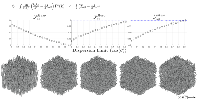
Simulations to test model assumptions were performed in Matlab. Cylinders were packed with various levels of dispersion (figure 4). Volume fractions around 15% were reached for solid fibers. Fibers were then hollowed after packing. $$$\mathcal{Y}_{\alpha\beta}^{Meso}$$$ was calculated numerically^6,7 and compared with eqn. 11.

Results

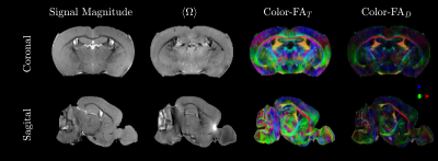
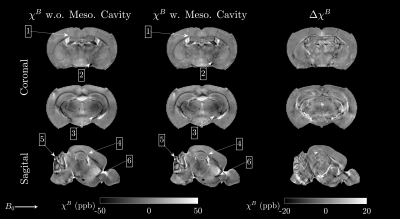
MRI data
Figure 2 gives an overview of the MGE signal magnitude, $$$\langle\Omega\rangle_k$$$ and color-coded FA of $$$T_{\alpha\beta}$$$ and diffusion tensor $$$D_{\alpha\beta}$$$. As expected,$$$T_{\alpha\beta}$$$ produced sharper colormaps than $$$D_{\alpha\beta}$$$. Figure 3 shows the susceptibility map $$$\chi^B$$$ from fitting eqn.13, with and without including $$$\langle\Omega\rangle^{Meso}_k$$$, along with the difference $$$\Delta\chi^B$$$.
Simulation
Validation of the macroscopic model assumptions for $$$\mathcal{Y}_{\alpha\beta}^{Macro}$$$ was previously presented¹¹. Figure 4 shows the diagonal of $$$\mathcal{Y}_{\alpha\beta}^{Meso}$$$ computed numerically, and from eqn. 11.

Discussion

It is clear from figure 4 that approximating $$$\mathcal{Y}_{\alpha\beta}^{Meso}$$$ based on the fODF is in excellent agreement with explicit numerical calculation. When fiber bundles are randomly oriented, $$$\langle\Omega\rangle^{Meso}_k$$$ is zero. As dispersion decreases, $$$\langle\Omega\rangle^{Meso}_k$$$ increases becoming maximal in the parallel limit.
It is also evident from the susceptibility maps in figure 3 that $$$\langle\Omega\rangle^{Meso}_k$$$ introduces noticeable changes in $$$\chi^B$$$. For example, at the isthmus of corpus callosum, the medial region is almost invisible without the mesoscopic contribution (as can be seen at point 1 and 5 in figure 3). Neglecting the mesoscopic contribution is analogous to classical QSM¹¹.
The model can also be extended to cylinders with a radially symmetric susceptibility tensor¹⁸. However, such a model would require sample rotations. Other limitations potentially affecting the accuracy of the model include the simple voxel shapes, and assumption of cylinders¹⁹. In addition, other types of inclusions could be needed to fully characterize the shift in Larmor frequency.

Conclusion

The first cumulant of the FID signal is considered as a probe of magnetic susceptibility in white matter. As a first step towards incorporation the fODF in order to bypass sample rotations, the local susceptibility is treated as a scalar. By fitting the model to MRI data from an ex-vivo mouse brain, a higher apparent resolution was achieved in susceptibility maps.

Acknowledgements

This study is funded by the Independent Research Fund (grant 8020-00158B), Denmark, and by Helga & Peter Korning's Foundation. The authors would like to thank PhD student Jonas Lynge Olesen for many fruitful discussions.