3965

Asymmetric Susceptibility Tensor Imaging

Steven Cao¹, Jingjia Chen¹, Hongjiang Wei², and Chunlei Liu¹
¹UC Berkeley, Berkeley, CA, United States, ²Shanghai Jiao Tong University, Shanghai, China

Synopsis

Susceptibility Tensor Imaging (STI) is a recently developed technique that uses phase data to solve for the underlying susceptibility tensor of the tissue. While STI has the potential for early diagnosis of many diseases including Parkinson’s and Alzheimer’s, it suffers from low image quality. From physics, the susceptibility tensor can be shown to be symmetric, so current approaches impose a symmetry constraint during inversion. We propose an inversion algorithm without this constraint, and instead enforce symmetry post-inversion by decomposing the result into symmetric and antisymmetric parts. We justify this approach empirically by comparing reconstructions of mouse brain and kidney data.

Introduction

Susceptibility Tensor Imaging (STI) is a recently developed MRI technique that measures anisotropic magnetic susceptibility with a tensor model (1). Scalar magnetic susceptibility measured in a single B0-field direction, achieved by a technique called Quantitative Susceptibility Mapping (QSM), has been shown to be sensitive to iron content, myelin, and collagen fibril organization, making it useful for the study of a multitude of diseases, including Parkinson’s, Alzheimer's, multiple sclerosis, fibrosis, and osteoarthritis (1,3,4,6,13,16,24-26). However, magnetic susceptibility is anisotropic in some tissues and therefore must be described by a tensor (1,5,8,17-20). Susceptibility tensor tractography has been shown to convey information about white matter tracts, kidney tubules, myofibers, and fibers not encapsulated by diffusion-based tractography (2,7,8,11,21).

Despite this promise, reconstruction of the susceptibility tensor from multi-orientation phase maps faces many challenges due to low SNR, especially in the off-diagonal terms, and vulnerability to streaking artifacts. Injection of a gadolinium-based contrast agent improves contrast (27), but at the cost of imaging artifacts in areas where the contrast agent accumulates and alteration of native susceptibility values. These problems distort underlying structures and make fiber tracking difficult. Multiple regularization schemes have been proposed to produce better tensor images (9-11,22,23). However, these schemes often rely on assumptions that are not true in general (e.g. only white matter being anisotropic (10)), and their increased SNR typically comes at the cost of significant blurring.

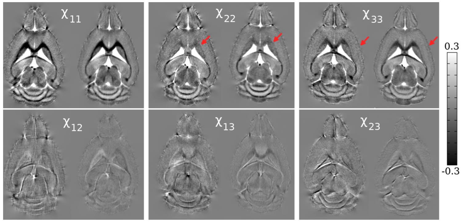
In contrast, in this study, we exploit the symmetry of the susceptibility tensor to present a new STI reconstruction algorithm that produces higher SNR and improved anatomical contrast without regularization. From physics, the susceptibility tensor can be shown to be symmetric, so current approaches impose a symmetry constraint during inversion (5). We propose an inversion algorithm without this constraint, termed asymmetric STI (aSTI), and instead enforce symmetry post-inversion by decomposing the result into symmetric and antisymmetric parts. We justify this approach empirically by comparing reconstructions of mouse brain and kidney data.

Theory

Given an applied field $$$\vec{B}_0 = B_0 \hat{H}$$$ with magnitude $$$B_0$$$ and direction $$$\hat{H}$$$, let $$$\mathbf{\chi}(\vec{x})$$$ denote the susceptibility tensor at each point $$$\vec{x}$$$. Then, the resulting frequency shift in the Fourier domain is given by
$$\Delta B_k (\vec{k}) = \hat{H}^T \left( \frac{1}{3} I - \frac{\vec{k} \vec{k}^T}{\vec{k}^T\vec{k}} \right) \mathbf{\chi_k}(\vec{k}) B_0 \hat{H},$$
where $$$\vec{k}$$$ denotes the point in the Fourier domain (5,6). This equation is linear in the 9 terms of $$$\mathbf{\chi_k}$$$. If we constrain $$$\mathbf{\chi_k}$$$ to be symmetric, we need to solve for 6 terms, so we can apply the magnetic field in $$$n \geq 6$$$ directions $$$\hat{H}_1,...,\hat{H}_6$$$ and invert the resulting $$$n$$$ linear equations via least squares.

In the case where $$$\mathbf{\chi_k}$$$ is not symmetric, we must solve for 9 terms; however, one can show that there are at most 6 linearly independent directions. Therefore, to invert, we choose the least squares solution with the minimum norm. Then, to impose the symmetry constraint, we decompose the tensor into the symmetric and antisymmetric parts $$$(\mathbf{\chi} + \mathbf{\chi}^T)/2$$$ and $$$(\mathbf{\chi} - \mathbf{\chi}^T)/2$$$.

Methods

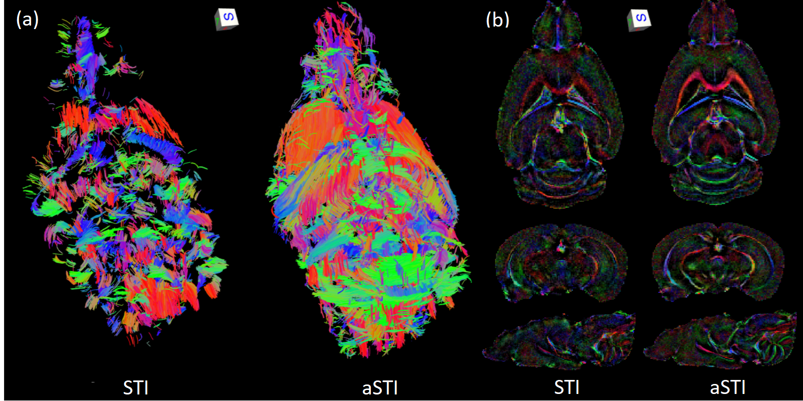
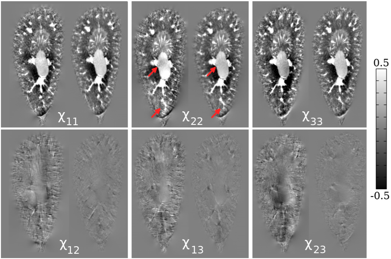
We obtain GRE phase data from postmortem mouse brain and kidney samples, rotated in 17 directions. Please see (11) for details about the data acquisition process. We then apply both symmetric and asymmetric tensor reconstructions to the data and compare the results.

The reconstructions are also used for STI fiber tracking: in the brain, we track white matter by tracking the smallest eigenvector direction (7), while in the kidney we track tubules by tracking the largest eigenvector direction (8). To identify which regions to track, we use the susceptibility index (9), which is given by
$$ SI = \frac{\chi_1 - \chi_3}{\chi_1 + \chi_2 + \chi_3}, $$
rescaled to be from 0 to 1, where $$$\chi_1 \geq \chi_2 \geq \chi_3$$$ are the three eigenvalues of the susceptibility tensor.

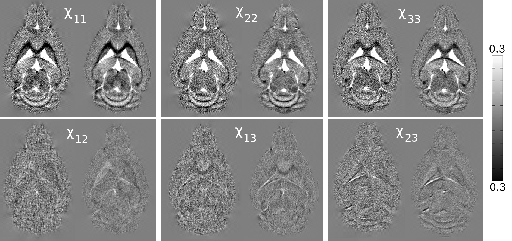
We also perform simulations with a ground truth to compare the methods quantitatively. Specifically, given a susceptibility tensor ground truth, we apply the forward model and add Gaussian noise at various noise levels. We then apply the reconstruction methods and compute mean squared error.

Results

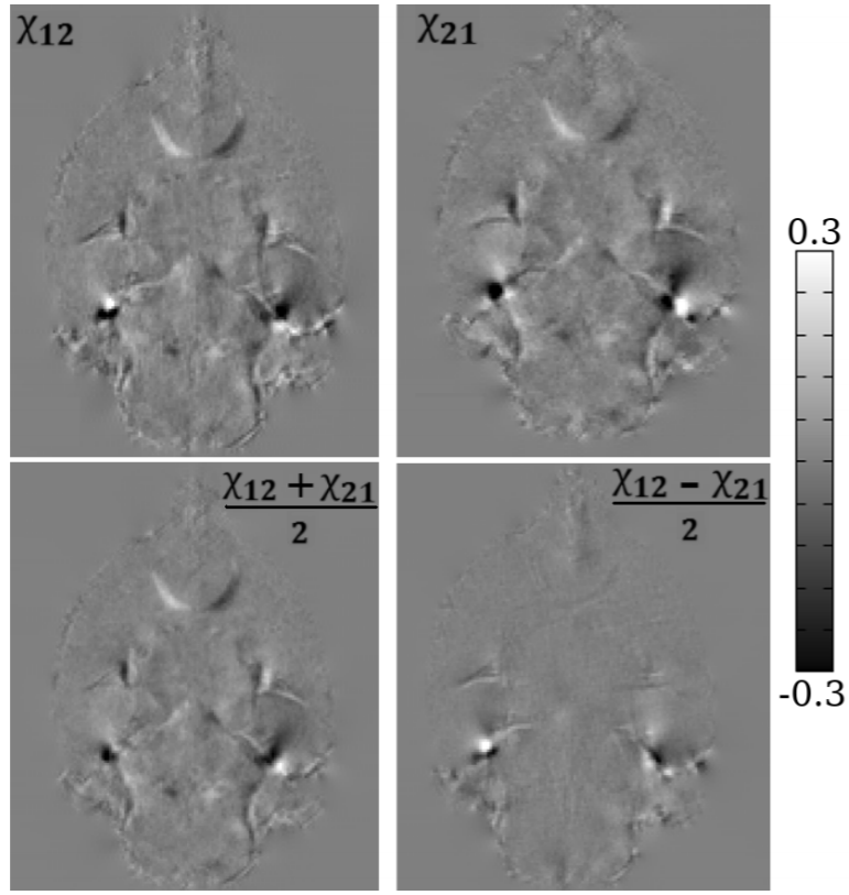
Compared to the symmetric reconstruction, the asymmetric reconstruction shows reduced noise and streaking artifacts, better contrast, and more complete fiber tracking (see Figures 1 and 3 for brain and kidney reconstructions, and Figure 2 for brain fiber tracking). In simulation, the asymmetric reconstruction achieves better mean squared error in the presence of noise. We also examine the simulated reconstructions in Figure 4, which confirms that the asymmetric reconstruction is less noisy.

Decomposing the asymmetric tensor into its symmetric and antisymmetric components, we see that the underlying susceptibility tensor is symmetric, and the main sources of asymmetry are noise and streaking artifacts (Figure 5). This observation provides one explanation for the method's success: because noise and artifacts do not follow the symmetry constraint, we can mitigate them by performing asymmetric reconstruction and removing the antisymmetric part afterward.

Conclusion

While the susceptibility tensor is symmetric, asymmetric reconstruction is more effective in suppressing noise and artifacts, resulting in more accurate estimation of the susceptibility tensor.

Acknowledgements

No acknowledgement found.

References

1. Langkammer et al., Quantitative susceptibility mapping (QSM) as a means to measure brain iron? A post mortem validation study, Neuroimage 2012.

2. Wei et al., Susceptibility tensor imaging and tractography of collagen fibrils in the articular cartilage, MRM 2017.

3. Wei et al., Quantitative susceptibility mapping of articular cartilage in patients with osteoarthritis at 3T, JMRI 2019.

4. Guan et al., Regionally progressive accumulation of iron in Parkinson’s disease as measured by quantitative susceptibility mapping, NMR Biomed 2017.

5. Liu, Susceptibility Tensor Imaging, MRM 2010.

6. Liu et al., Susceptibility-Weighted Imaging and Quantitative Susceptibility Mapping in the Brain, JMRI 2015.

7. Li et al., Magnetic susceptibility anisotropy of human brain in vivo and its molecular underpinnings, Neuroimage 2012.

8. Xie et al., Susceptibility tensor imaging of the kidney and its microstructural underpinnings, MRM 2015.

9. Liu et al., 3D fiber tractography with susceptibility tensor imaging, Neuroimage 2012.

10. Li et al., Mean Magnetic Susceptibility Regularized Susceptibility Tensor Imaging (MMSRSTI) for Estimating Orientations of White Matter Fibers in Human Brain, MRM 2015.

11. Dibb et al., Joint Eigenvector Estimation from Mutually Anisotropic Tensors Improves Susceptibility Tensor Imaging of the Brain, Kidney, and Heart, MRM 2017.

12. Ruopeng Wang, Van J. Wedeen, TrackVis.org, Martinos Center for Biomedical Imaging, Massachusetts General Hospital

13. Acosta-Cabronero J, Williams GB, Cardenas-Blanco A, Arnold RJ, Lupson V, Nestor PJ, In vivo quantitative susceptibility mapping (QSM) in Alzheimer's disease, PLoS One, 2013.

14. Johnson GA, Cofer GP, Gewalt SL, Hedlund LW. Morphologic phenotyping with MR microscopy: the visible mouse. Radiology. 2002;222(3):789–793.

15. Li W, Avram AV, Wu B, Xiao X, Liu C. Integrated Laplacian-based phase unwrapping and background phase removal for quantitative susceptibility mapping. NMR Biomed. 2014;27(2):219–227.

16. Xie, Luke, et al. "Quantitative susceptibility mapping of kidney inflammation and fibrosis in type 1 angiotensin receptor‐deficient mice." NMR in biomedicine 26.12 (2013): 1853-1863.

17. Lee, Jongho, et al. "Sensitivity of MRI resonance frequency to the orientation of brain tissue microstructure." Proceedings of the National Academy of Sciences 107.11 (2010): 5130-5135.

18. Wei, Hongjiang, et al. "Imaging diamagnetic susceptibility of collagen in hepatic fibrosis using susceptibility tensor imaging." Magnetic Resonance in Medicine 83.4 (2020): 1322-1330.

19. Bilgic, Berkin, et al. "Rapid multi-orientation quantitative susceptibility mapping." NeuroImage 100.125 (2016): 1131-1141.

20. Dibb, Russell, Yi Qi, and Chunlei Liu. "Magnetic susceptibility anisotropy of myocardium imaged by cardiovascular magnetic resonance reflects the anisotropy of myocardial filament α-helix polypeptide bonds." Journal of Cardiovascular Magnetic Resonance 17.1 (2015): 1-14.

21. Liu, Chunlei, et al. "3D fiber tractography with susceptibility tensor imaging." Neuroimage 59.2 (2012): 1290-1298.

22. Wisnieff, Cynthia, et al. "Magnetic susceptibility anisotropy: cylindrical symmetry from macroscopically ordered anisotropic molecules and accuracy of MRI measurements using few orientations." Neuroimage 70 (2013): 363-376.

23. Li, Xu, et al. "Mapping magnetic susceptibility anisotropies of white matter in vivo in the human brain at 7 T." Neuroimage 62.1 (2012): 314-330.

24. Langkammer, Christian, et al. "Quantitative susceptibility mapping in multiple sclerosis." Radiology 267.2 (2013): 551-559.

25. Wisnieff, Cynthia, et al. "Quantitative susceptibility mapping (QSM) of white matter multiple sclerosis lesions: interpreting positive susceptibility and the presence of iron." Magnetic resonance in medicine 74.2 (2015): 564-570.

26. Wei, Hongjiang, et al. "Investigating magnetic susceptibility of human knee joint at 7 Tesla." Magnetic resonance in medicine78.5 (2017): 1933-1943.

27. Dibb, Russell, et al. "Microstructural origins of gadolinium‐enhanced susceptibility contrast and anisotropy." Magnetic resonance in medicine 72.6 (2014): 1702-1711.

28. Hinoda, Takuya, et al. "Quantitative susceptibility mapping at 3 T and 1.5 T: evaluation of consistency and reproducibility." Investigative radiology 50.8 (2015): 522-530.

Figures

The susceptibility tensor reconstructions of the mouse brain (left: STI, right: aSTI, color scale: -0.3 to 0.3 ppm). The aSTI results show the symmetric component of the reconstructed asymmetric tensor, and similarly for other figures. In all six terms, the aSTI reconstruction has less noise and better contrast. The red arrow on χ₂₂ shows improved delineation of the corpus callosum. The red arrow on χ₃₃ shows improved separation between the cortical layers, where the outer layer has a clear stripe of lower susceptibility.

(a) Fiber tracking results of the minor eigenvector, where fibers shorter than 5mm are not shown (left: STI, right: aSTI). The aSTI reconstruction recovers much more of the white matter fiber tracks. (b) The minor eigenvector direction of the mouse brain, weighted by SI (left: STI, right: aSTI). The aSTI color maps show more coherent fiber directions, and the SI also serves as a better indicator of white matter.

The susceptibility tensor reconstructions of the mouse kidney (left: STI, right: aSTI, color scale: -0.5 to 0.5 ppm). In the off-diagonal terms of the STI reconstruction, we see artifacts in the form of light and dark streaks that are not present in the aSTI reconstruction. The lower red arrows in χ₂₂ show that in the STI reconstruction, the high susceptibility of the blood vessels bleeds into neighboring areas. The upper red arrows show an area in the renal pelvis with a dark spot where the susceptibility should be uniform.

The susceptibility tensor reconstructions of the mouse brain using simulated phase with 5% additive white Gaussian noise (left: STI, right: aSTI, color scale: -0.3 to 0.3 ppm). The aSTI reconstruction has greatly reduced noise. Also, the off-diagonal terms are lower in amplitude and closer to the ground truth in the aSTI reconstruction compared to the STI reconstruction, verifying the reduced magnitude in the aSTI reconstructions of real phase data (see Figures 1 and 3).

The χ₁₂ (top left) and χ₂₁ (top right) terms in the aSTI reconstruction, along with the symmetric (bottom left) and antisymmetric (bottom right) decompositions. The antisymmetric part contains mostly noise and streaking artifacts. As a result, after discarding the antisymmetric part, the symmetric part shows reduced noise and streaking compared to the top two images.

Proc. Intl. Soc. Mag. Reson. Med. 29 (2021)

3965