3961
RF Pulse Designs for Velocity-Selective MRA at Low Field Strengths1Ming Hsieh Department of Electrical and Computer Engineering, Viterbi School of Engineering, University of Southern California, Los Angeles, CA, United States, 2Department of Biomedical Engineering, Viterbi School of Engineering, University of Southern California, Los Angeles, CA, United States
Synopsis
Velocity‐selective (VS) RF pulses can differentiate flowing blood from background tissue, and have been utilized for non-contrast intracranial, abdominal, and peripheral angiography at 3T. Here, we explore RF pulse designs for intracranial VS-MRA at low field strengths including 0.55T. We evaluate pulse performance using simulations that incorporate realistic levels of B0 variation, B1+ variation, and gradient distortions. Compared to 3T, simulations indicate 22% - 38% sharper velocity transitions and/or 50% - 60% less signal loss at 0.55T. We also show that gradient distortions can lead to “stripe” artifacts and can be mitigated with pre-emphasis.
INTRODUCTION
Velocity-selective (VS) RF pulses provide a novel mechanism for generating contrast between flowing blood and background tissue.1 VS pulses have been extensively applied to non-contrast MR angiography of the brain,2.3 abdomen,4 and peripheral vasculature 5,6 at 3T. The design of VS pulses must consider B0 and B1+ inhomogeneity 2,7 and eddy currents .5,8 These have been addressed at 3T, with solutions requiring longer pulse duration that leads to increased T2 related signal loss. Lower field strengths, including 0.55T, are expected to provide greater flexibility in VS pulse design due to the improved B0 and B1+ homogeneity, and relaxed SAR constraints. Here, we simulate the performance of VS pulses for intracranial VS-MRA at 0.55T and 3T, taking into account of realistic B0 and B1+ variation and gradient imperfections.METHODS
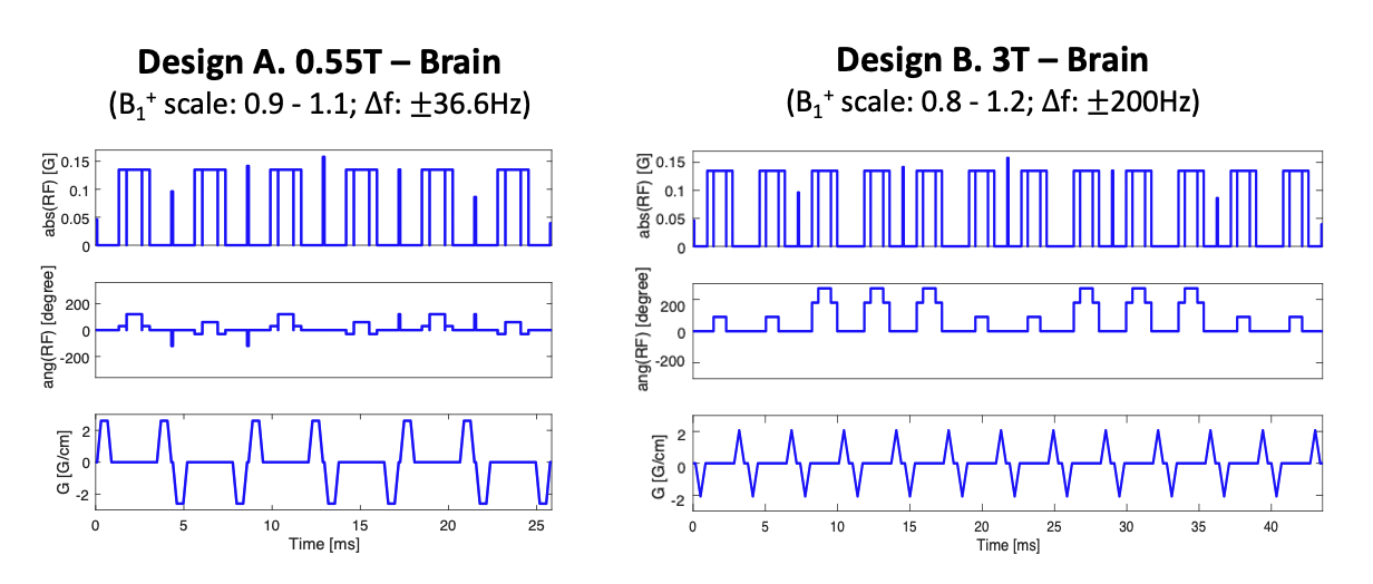
Velocity Selection for Intracranial MRA. VS pulses were designed to saturate the velocity range from -0.5 to 0.5cm/s and to have minimal impact on spins from 11.5 to 33.5 cm/s. The velocity field of view (FOVv) was set to 45cm/s in order to cover the flow velocity of major cerebral arteries (30 - 40cm/s).9 The time bandwidth product was set to 1.8 for all designs. Physiologic T1 and T2 values of arterial blood were used for Bloch simulations: T1/T2=1121/263 ms at 0.55T10; and 1650/150 ms at 3T.11,12 We report the cutoff velocity which represents the transition sharpness for the excitation profile on-resonance and with B1+ scale=1.VS pulse design. We designed VS pulse trains to achieve similar performance under realistic levels of B0 and B1+ variation. We selected single refocused pulse trains for 0.55T.7 We selected paired refocused pulse trains with MLEV phase cycling for 3T.13 Composite refocusing pulses (90x-180y-90x) were used for both field strengths. The RF sub-pulse envelope was designed using the Shinnar-Le Roux transform.14 We tested 5 to 17 sub-pulses (4-16 kv steps) at 0.55T, and 5 to 9 sub-pulses (4-8 kv steps) at 3T. Figure 1 contains two representative pulses.
B0/B1+ variation consideration. We used a range of ±200 Hz for off-resonance at 3T and an adjusted range of ±36.6 Hz at 0.55T since B0 variation is proportional to the field strength.15 B1+ scale varied from 0.8 to 1.2 at 3T 16 and 0.9 to 1.1 at 0.55T.17
Gradient performance and imperfection. Gradient waveforms were designed for a maximum 40 mT/m amplitude and 200 mT/m/ms slew rate. We use gradient impulse response functions (GIRFs) from a published dataset 18 to examine performance with distortion and with GIRF-based pre-compensation.19,20
RESULTS
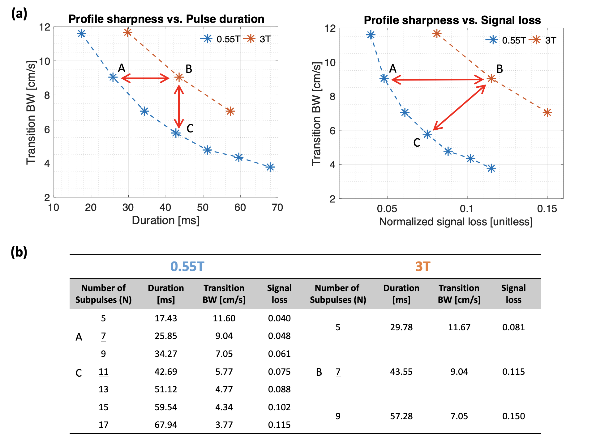
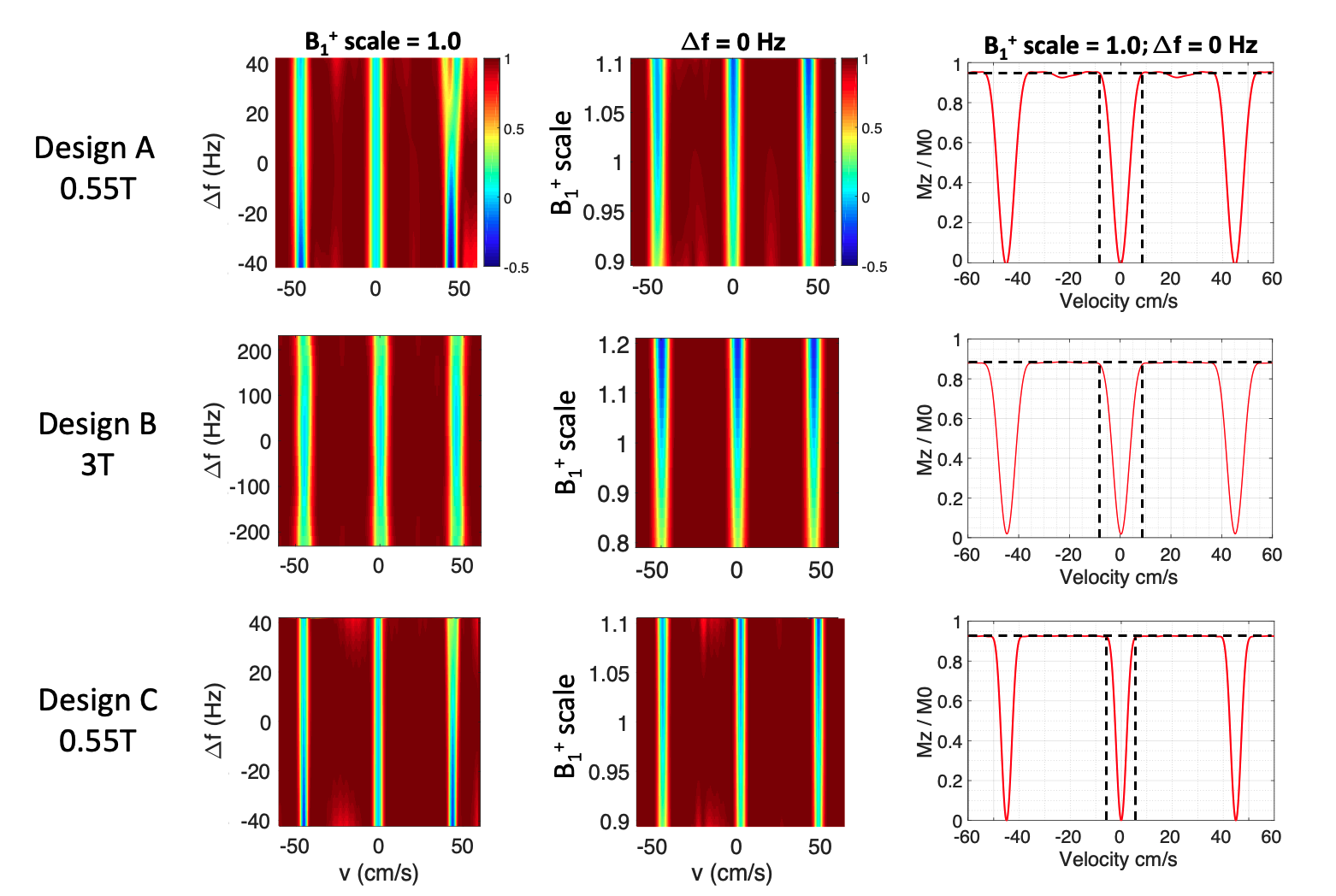
Figure 2 (a) demonstrates the tradeoffs between pulse duration (left), or equivalently signal loss (right) and velocity sharpness at 0.55T and 3T. The designed pulses at 0.55T (blue), compared with the 3T (orange), have better fidelities over the tradeoffs between transition bands and duration or signal loss. 1) With the same transition widths (design A and B), the designs at 0.55T achieve roughly 40% shorter durations than designs at 3T (left) and achieve 50 - 60% reduced signal loss (right). 2) With similar pulse durations (design B and C), the designs at 0.55T achieve 22 - 38% sharper transitions (left) and have 35% less signal loss (right).Figure 3 demonstrates the Mz velocity profiles under off-resonance effects and B1+ inhomogeneity at 0.55T (Design A and C) and 3T (Design B). Profiles with relaxation effects under $$$\Delta$$$f = 0 Hz and B1+ scale = 1.0 are plotted on the right. Overall, the pulse profiles at 0.55T and 3T under off-resonance (1st column) and B1+ variation (2nd column) have similar patterns and can be comparable. 1) Design A and B achieve same transition bands whereas B has more signal loss (black dashed lines in 3rd column). 2) Design B and C achieve the same pulse durations, but C has sharper transitions as well as less signal loss (black dashed lines in 3rd column).
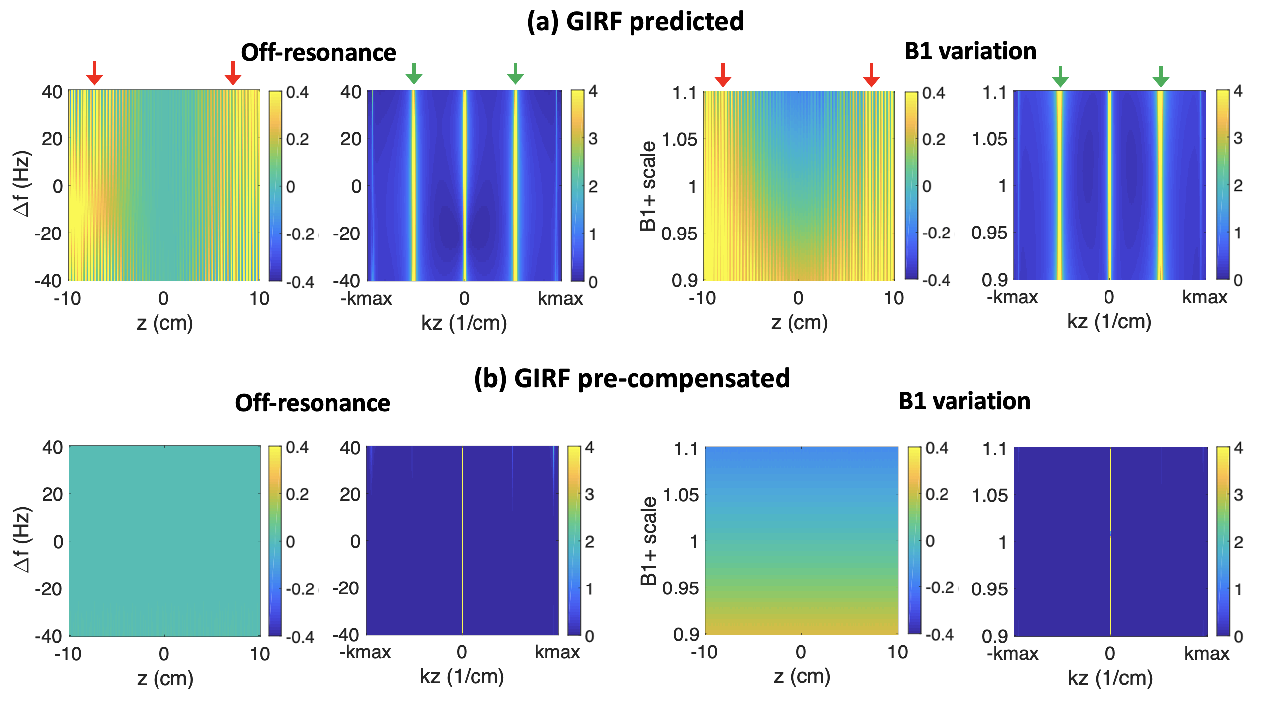
Figure 4 shows stripe artifacts of design A at 0.55T. (a) GIRF-predicted gradients generate enhanced signal modulations in the spatial domain (red arrows in 1st and 3rd columns) and spurious peaks in the frequency domain (green arrows in 2nd and 4th columns) across off-resonance and B1+ variations. (b) With gradient pre-emphasis based on GIRFs, the spatial profiles become almost uniform and the peaks are successfully saturated in the frequency domain.
DISCUSSION
Future work includes in-vivo validation and optimization of VS-MRA imaging methods, which should be reconsidered due to shorter T1 and longer T2 at low-field. We also plan to explore concomitant fields effects, which are more prominent at low-field and may deteriorate performance.21 Similar pulses may improve other VS-MRA applications, each with unique considerations (e.g. FOV, FOVv, velocity cutoffs, B1+ variation).CONCLUSION
Lower field strengths provide improved B0 and B1+ homogeneity compared to conventional field strengths. In the context of VS-MRA, our simulations indicate this could translate to 50 - 60% less signal loss (partially recovering the SNR loss due to reduced polarization) and/or 22 - 38% sharper velocity selection (potentially improving visualization of slow flow and/or distal vessels). Enhanced stripe artifacts due to gradient distortions can be mitigated with gradient pre-emphasis based on GIRFs.Acknowledgements
This work was supported by NSF Grant #1828736.References
1. De Rochefort L, Maître X, Bittoun J, Durand E. Velocity-selective RF pulses in MRI. Magn. Reson. Med. 2006;55:171–176.
2. Qin Q, Shin T, Schär M, Guo H, Chen H, Qiao Y. Velocity-selective magnetization-prepared non-contrast-enhanced cerebral MR angiography at 3 Tesla: Improved immunity to B0/B1 inhomogeneity. Magn. Reson. Med. 2016;75:1232–1241.
3. Li W, Xu F, Schär M, et al. Whole-brain arteriography and venography: Using improved velocity-selective saturation pulse trains. Magn. Reson. Med. 2018;79:2014–2023.
4. Zhu D, Li W, Liu D, et al. Non-contrast-enhanced abdominal MRA at 3 T using velocity-selective pulse trains. Magn. Reson. Med. 2020;84:1173–1183.
5. Shin T, Qin Q, Park JY, Crawford RS, Rajagopalan S. Identification and reduction of image artifacts in non–contrast-enhanced velocity-selective peripheral angiography at 3T. Magn. Reson. Med. 2016;76:466–477.
6. Shin T, Menon RG, Thomas RB, et al. Unenhanced Velocity-Selective MR Angiography (VS-MRA): Initial Clinical Evaluation in Patients With Peripheral Artery Disease. J. Magn. Reson. Imaging 2019;49:744–751.
7. Shin T, Hu BS, Nishimura DG. Off-resonance-robust velocity-selective magnetization preparation for non-contrast-enhanced peripheral MR angiography. Magn. Reson. Med. 2013;70:1229–1240.
8. Shin T, Qin Q. Characterization and suppression of stripe artifact in velocity-selective magnetization-prepared unenhanced MR angiography. Magn. Reson. Med. 2018;80:1997–2005.
9. Meckel S, Leitner L, Bonati LH, et al. Intracranial artery velocity measurement using 4D PC MRI at 3 T: Comparison with transcranial ultrasound techniques and 2D PC MRI. Neuroradiology 2013;55:389–398.
10. Campbell-Washburn AE, Ramasawmy R, Restivo MC, et al. Opportunities in interventional and diagnostic imaging by using high-performance low-field-strength MRI. Radiology 2019;293:384–393.
11. Zhang X, Petersen ET, Ghariq E, et al. In vivo blood T1 measurements at 1.5 T, 3 T, and 7 T. Magn. Reson. Med. 2013;70:1082–1086.
12. Lu H, Xu F, Grgac K, Liu P, Qin Q, Van Zijl P. Calibration and validation of TRUST MRI for the estimation of cerebral blood oxygenation. Magn. Reson. Med. 2012;67:42–49.
13. Jacobs JWM, Van Os JWM, Veeman WS. Broadband heteronuclear decoupling. J. Magn. Reson. 1983;51:56–66.
14. Pauly J, Nishimura D, Macovski A, Roux P Le. Parameter Relations for the Shinnar-Le Roux Selective Excitation Pulse Design Algorithm. IEEE Trans. Med. Imaging 1991;10:53–65.
15. Farahani K, Sinha U, Sinha S, Chiu LCL, Lufkin RB. Effect of field strength on susceptibility artifacts in magnetic resonance imaging. Comput. Med. Imaging Graph. 1990;14:409–413.
16. Bliesener Y, Zhong X, Guo Y, et al. Radiofrequency transmit calibration: A multi-center evaluation of vendor-provided radiofrequency transmit mapping methods. Med. Phys. 2019;46:2629–2637.
17. Campbell-washburn AE, Jiang Y, Körzdörfer G, Nittka M, Griswold MA. Feasibility of MR fingerprinting using a high-performance 0 . 55T MRI system. Proc. ISMRM 28th Sci. Sess. 2020:0868.
18. Çavuşoğlu M, Mooiweer R, Pruessmann KP, Malik SJ. VERSE-guided parallel RF excitations using dynamic field correction. NMR Biomed. 2017;30:1–13.
19. Stich M, Wech T, Slawig A, et al. Gradient waveform pre-emphasis based on the gradient system transfer function. Magn. Reson. Med. 2018;80:1521–1532.
20. Vannesjo SJ, Duerst Y, Vionnet L, et al. Gradient and shim pre-emphasis by inversion of a linear time-invariant system model. Magn. Reson. Med. 2017;78:1607–1622.
21. Bernstein MA, Zhou XJ, Polzin JA, et al. Concomitant gradient terms in phase contrast MR: Analysis and correction. Magn. Reson. Med. 1998;39:300–308.
Figures