3930
3D bSSFP Imaging performance using high performance gradients at 0.5T is comparable to standard field strengths: Clinical use in Temporal Bone MRI
David Volders1, James Rioux1, Steven Beyea1, Chris V Bowen2, and Elena Adela Cora1
1Diagnostic Radiology, Nova Scotia Health, Halifax, NS, Canada, 2Diagnostic Imaging, Nova Scotia Health, Halifax, NS, Canada
1Diagnostic Radiology, Nova Scotia Health, Halifax, NS, Canada, 2Diagnostic Imaging, Nova Scotia Health, Halifax, NS, Canada
Synopsis
Evaluation of temporal bone MRI scans using a 0.5T high performance gradient head only system reveals high quality visualization of clinically relevant structures using 3D bSSFP imaging.
INTRODUCTION
MRI of the temporal bone is a well-established clinical tool for evaluating pathology in small structures at high resolution. Traditionally this favors high field strength imaging due to the SNR advantages, however the temporal bone is a challenging region for susceptibility artifact with numerous air/bone/tissue interfaces, often leading to the use of 3D FSE rather than more SNR efficient sequences, like bSSFP, for artifact suppression considerations [1].We postulated that a novel, head-only, 0.5T EvryTM system [2], with its combination of high-performance imaging gradients and low field strength, might produce comparable image quality to higher field clinical systems, due to the reduction of susceptibility banding artifacts common in bSSFP [3]. We recruited patients having routine temporal bone clinical MRI scans for an additional 0.5T MRI scan and had 2 board certified neuro-radiologists evaluate 5 anatomic structures of clinical relevance using a 5-point Likert scale.
Our aim was to demonstrate image quality for 0.5T bSSFP acquisitions that were non-inferior to clinical field strength acquisitions, assessed through radiologist assessment of relevant anatomic features in temporal bone MRI scans.
METHODS
Data were acquired from six patients who had previously undergone clinical temporal bone MRI scans involving bSSFP acquisitions. Following completion of their clinical scan, patients were scanned on the EvryTM system [2] under a NSH REB-approved protocol. The protocol we developed used an axial 3D balanced-SSFP acquisition with 0.6mm isotropic resolution interpolated onto a 0.3mm isotropic reconstruction matrix.Scan parameters selected were 18cm FOV, 300x300, 1NEX, 0.6mm slice thickness, 164 slices, 70kHz RBW, TR/TE 6.73/3.3ms, flip-angle 60 (Scan time 4 min 19 s). The unique head-only gradient set for this system performs imaging at the outer Z-direction edge of the gradient coil, without shoulders/lower body inserted. This enables very high slew rate (400 T/m/s) and gradient strength (9 g/cm) performance, which we operated conservatively at SR 200 T/m/s and 6 g/cm for this study. Clinical systems with whole-body gradients typically operate with much lower SR (~140 T/m/s) due do peripheral nerve stimulation constraints that are not relevant for this configuration (PNS has never been reported on this system at our site). The low patient heating SAR inherent at 0.5T enabled high flip angle b-SSFP acquisitions with short TR, while the high SR performance gradients enabled short TR with high receiver-on duty cycle for maximum SNR efficiency. The superior Bo field homogeneity at 0.5T enabled relatively longer TR values without banding artifacts for bSSFP acquisitions, making it ideal for use in this application. De-identified clinical images for each patient were obtained at either 3T (3) or 1.5T (3), with bSSFP acquisitions having isotropic resolution of 0.6mm (3T) or 0.8mm (1.5T), interpolated onto a similar resolution matrix as our 0.5T acquisitions.
All bSSFP images were shown to two board-certified neuro-radiologists who were asked to rate image quality for 5 anatomic structures of relevance to clinical temporal bone MRI exams [1] (see Table 1). A 1-5 Likert scale was used (1-5 ranging from very poor to excellent) and scoring was separately recorded for each ear. Since blinding to field strength is not practical, due to unique IQ features, we presented the 0.5T images first for scoring, with clinical images second, since many of these patients have existing pathologies that we eventually hope to perform a diagnostic sensitivity analysis upon (as more patients receive scans).
RESULTS AND DISCUSSION
Figure 1a and 1b show representative cross-sectional images from a patient at 0.5T and at 3T (clinical scan), respectively. The 5 relevant structures rated for image quality (see Table 1) are shown via arrows in each figure (see caption). Since all acquisitions are isotropic resolution, they are easily amenable to re-sectioning for visualization.Table 1 shows the mean and standard deviation for each Likert scale averaged over both ears and each radiologist separated into overall score, as well as individual scoring for each of the 5 anatomic structures investigated. The group mean Likert score overall, as well as that for each of the 5 structures was higher for 0.5T than clinical scans. A 1-tailed paired t-test of scores for each structure, and by each radiologist, comparing the 0.5T and clinical scanner is also shown in Table 1. A significant improvement at the p<0.05 threshold was observed for the overall score, as well as for the semi-circular canals (SSC), and vestibulum. The other 3 structures (cochlea, cochlear nerve and facial nerve) had higher mean Likert scores, but failed to reach significance at p<0.05.
The 0.5T scans qualitatively appear to better resolve structures, without artifact, with a grainier (low SNR) appearance. This may explain the improved visualization of small structures with inherently fine detail (SSC, vestibulum) while larger structures with low contrast-to-noise are more equivocal (nerves in particular).
CONCLUSIONS AND FUTURE WORK
This study demonstrates that a head-only low-field, point-of-care MRI system with high-performance gradients may be ideally suited to resolving fine structures at high resolution. While general trends have been observed, future work will include a larger data set, with evaluation of pathology visualization, such that a sensitivity analysis to a variety of pathologies encountered in temporal bone MRI exams can be determined. If successful, this may enable express, non-contrast enhanced temporal bone MRI scans for clinical use.Acknowledgements
Funding for this research was provided by grants from Research Nova Scotia, NSERC Discovery program and Brain Repair Centre Knowledge Translation program.References
1. Benson JC, Carlson ML, Lane JI, MRI of the Internal Auditory Canal, Labyrinth, and Middle Ear: How We Do It, Radiology 2020; 297:252–265.
2. Stainsby JA, Bindseil GA, Connell IRO, Thevathasan G, Curtis AT, Beatty PJ, Harris CT, Wiens CN, and Panther A. Imaging at 0.5 T with high-performance system components. Proc. ISMRM 2019, no.1194.
3. Bowen CV, Gati JG, Menon RS, Robust prescan calibration for multiple spin-echo sequences: application to FSE and b-SSFP. MRI, 2006, 24(7):857-67.
Figures
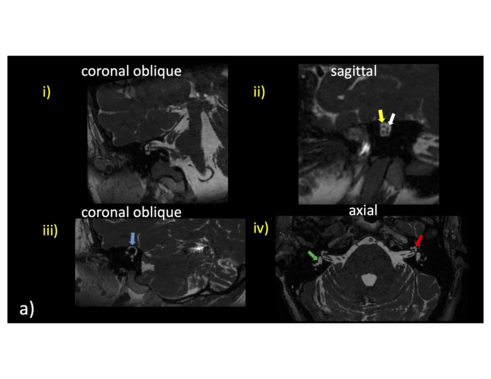
Figure 1: Representative cross-sectional 3D bSSFP images for a patient at 0.5T (a) and 3T (b) reformatted into various labeled planes (i.-iv.). Key anatomical structures being rated by 2 board certified radiologists are shown. Blue arrow: superior semicircular canal; Yellow arrow: facial (top) and cochear (bottom) nerve; White arrow: superior vestibular (top) and inferior vestibular (bottom) nerve; Green arrow: vestibule; Red arrow: cochlea.
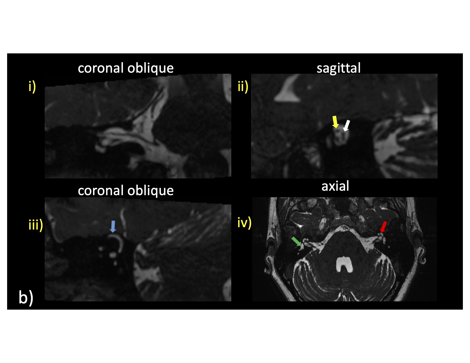
Figure 1: Representative cross-sectional 3D bSSFP images for a patient at 0.5T (a) and 3T (b) reformatted into various labeled planes (i.-iv.). Key anatomical structures being rated by 2 board certified radiologists are shown. Blue arrow: superior semicircular canal; Yellow arrow: facial (top) and cochear (bottom) nerve; White arrow: superior vestibular (top) and inferior vestibular (bottom) nerve; Green arrow: vestibule; Red arrow: cochlea.
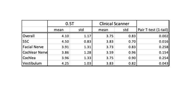
Table 1: Statistical comparison of 0.5T vs clinical field strength scans