Introduction

Glioblastomas are highly heterogeneous tumors, and optimal treatment depends on identifying and locating the highest grade disease present¹. Traditional non-invasive Glioblastoma grading is based on kinetic modeling of DCE-MRI data, which suffers from low sensitivity and a dependency on the choice of arterial input function (AIF) choice². To address the AIF problem of traditional kinetic modeling, recently a new method was recently proposed to model the contrast agent concentration change in space and time using transport equation without the requirement of AIF³. The blood flow can be calculated by inverting the transport equation, which is termed as quantitative transport mapping (QTM). In this work, we propose to evaluate the clinical value of QTM in glioblastoma grading by comparing with traditional kinetic modeling method.

Methods

QTM Algorithm: We use the transport equation to model the transport of tracers²: $$\partial _{t} c(\xi,t)=-\nabla\cdot c(\xi,t) u(\xi) \qquad (1)$$ where $$$c(\xi,t)$$$ is the tracer concentration in a voxel $$$\xi$$$,$$$\nabla$$$the spatial gradient, and $$$u(\xi)$$$ the average velocity in that voxel. Rewriting Eq.1 as $$$A\overrightarrow u = \overrightarrow b$$$ , where A is a large sparse matrix, $$$\overrightarrow u$$$ a large vector concatenating $$$u(\xi)$$$ for all voxels, and $$$\overrightarrow b$$$ a large vector concatenating $$$c(\xi,t)$$$ for all voxels and all time points. The inverse problem of reconstructing the velocity field $$$\overrightarrow u$$$ is formulated as a constrained minimization problem:$$\overrightarrow u = argmin_{\overrightarrow u} ||A\overrightarrow u-\overrightarrow b||_{2}^{2}+\lambda||\nabla \overrightarrow u||_{1} \qquad (2)$$ An L1 regularization is added in Eq.2 for denoising with $$$\lambda=10^{-3}$$$ chosen empirically according to minimal mean square error with respect to the ground truth for the simulation and image quality and L-curve characteristics for the in vivo data.
In vivo DCE MRI: 30 patients with glioblastoma were imaged using a T1-weighted 3D MRI sequence before and after the injection of gadolinium contrast agent using the following parameters: 0.94*0.94*5 mm³ voxel size, 256*256*16-34 matrix, 13-25° flip angle, 1.21 ms TE, 4.37ms TR, 6.2 s temporal resolution, and 30 time points. The grading of the tumor is determined based on surgery result. 15 of them are high grade (grading III or IV) and 15 of them are low grade (grading I or II). A ROI is drown on the whole tumor based on T1 DCE-MRI and T2 FLAIR imaging for statistic analysis. QTM processing by Eq.2 was performed on all data. The DCE 4D image data was converted to gadolinium concentration ([Gd]) data by assuming a linear relationship between signal intensity change and contrast agent concentration⁴. The velocity amplitude of each voxel was calculated as follows:
$$ |\boldsymbol{u}(\xi)|=\sqrt{(u^x(\xi))^2+(u^y(\xi))^2+(u^z(\xi))^2} \qquad (3) $$
$$$K^{trans}$$$ and $$$V_e$$$ were also obtained using Tofts’ model:
$$ \partial_tc(\xi,t)=k^{trans}(\xi)[c_a(t)-c(\xi,t)/V_e(\xi)] \qquad (4) $$
where $$$c_a(t)$$$was the global arterial input function (AIF). Two artery inputs are used, one acquired from carotid artery and another from the feeding artery of the tumor.
Statistical Analysis: A Receiver Operating Characteristic (ROC) curve was constructed for each parameter to characterize its performance in distinguishing between low (grade I, II) and high grade (grade III, IV) glioblastomas.

Results:

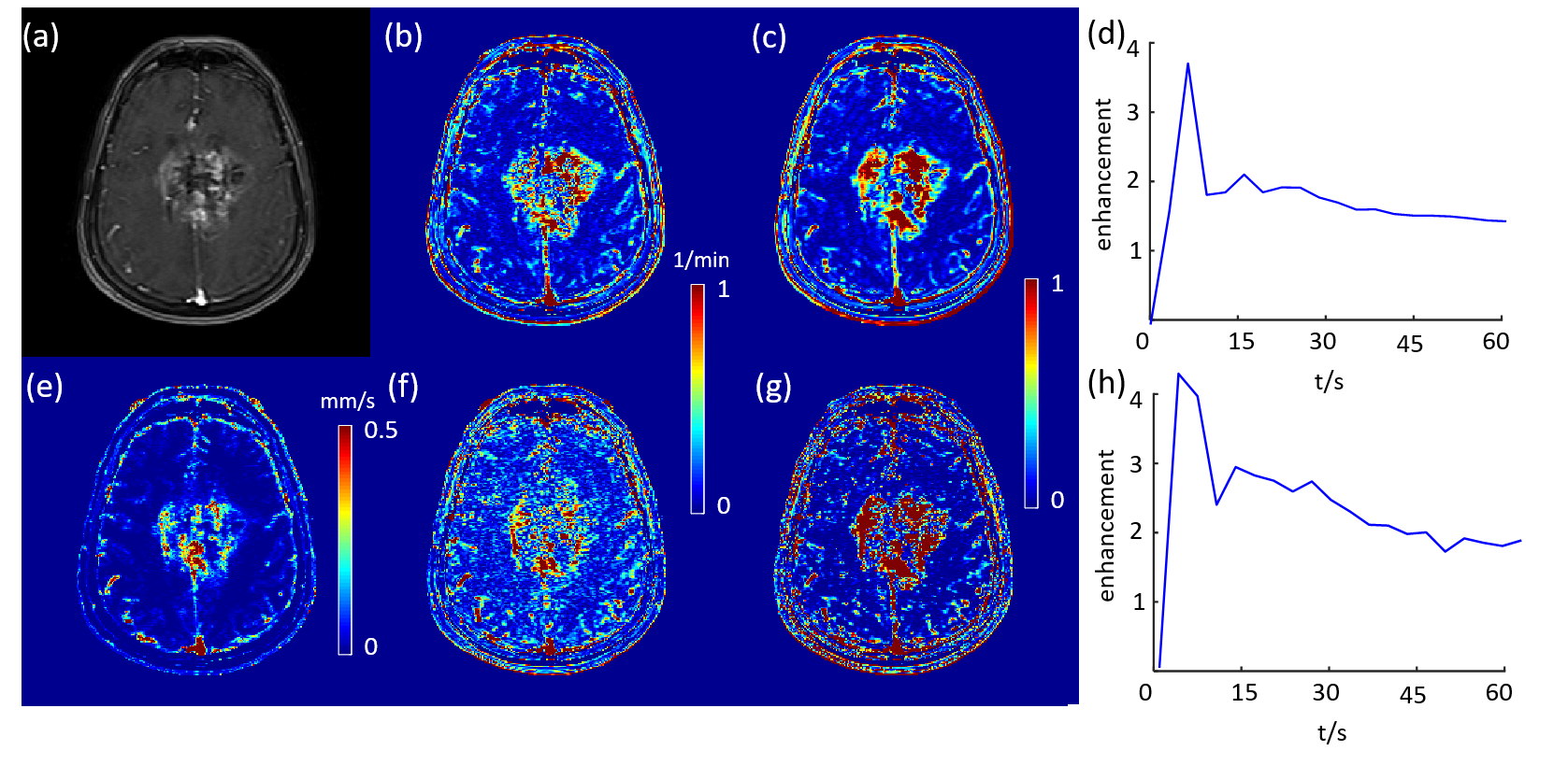
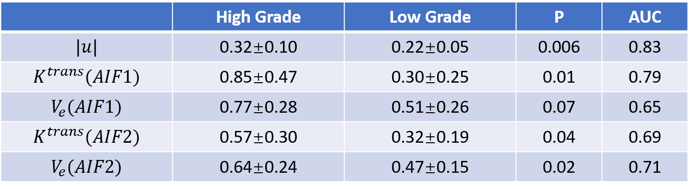
$$$\boldsymbol{u}$$$, $$$k^{trans}$$$and $$$V_e$$$ maps of a high grade glioblastoma tumor and a low grade glioblastoma tumor are shown in Figure 1 and 2, accordingly. The tumor is clearly shown on both $$$\boldsymbol{u}$$$ and $$$k^{trans}$$$ maps. However, the kinetic modeling result showed 30% difference using two different AIFs, which is consistent with a previous study². Among $$$\boldsymbol{u}$$$, $$$k^{trans}$$$and $$$V_e$$$ calculated using two different AIFs, U showed the best performance in distinguishing high grade and low grade glioblastoma (AUC=0.83), shown in Figure 3. AIF selected near the tumor showed better classification accuracy than AIF selected in carotid artery.

Discussion and Conclusion:

Compared with traditional kinetic modeling method, the QTM derived velocity showed the best classification performance grading glioblastomas. $$$k^{trans}$$$ and $$$V_e$$$ calculated using extended Toft’s model highly depended on the choice of AIF. Future work may include increasing the size of the dataset and comparing the performance of QTM and kinetic modeling method in differentiating glioblastoma of different grade (grades I,II,III and IV).

Acknowledgements

We don't have any acknowledgements.