3849
Stereological Modeling of Hepatic Steatosis and Estimating Independent R2* for Water and Fat using Monte Carlo Simulations1Biomedical Engineering, The University of Memphis, Memphis, TN, United States, 2College of Health Sciences, The University of Memphis, Memphis, TN, United States, 3Computer Science, The University of Memphis, Memphis, TN, United States, 4Electrical & Computer Engineering, The University of Memphis, Memphis, TN, United States, 5North Shore University Hospital/Northwell Health, Manhasset, NY, United States, 6St. Jude Children’s Research Hospital, Memphis, TN, United States
Synopsis
Multi-spectral fat-water models assume either single or independent R2* for water (R2*W) and fat (R2*F) for assessment of steatosis. However, any incorrect assumptions in the signal model will produce errors in R2* and fat fraction (FF) calculations. In this study, we developed a Monte Carlo–based approach for generating steatosis models by characterizing fat morphology from histology and synthesizing MRI signal to estimate independent R2*W and R2*F and compare with in-vivo studies. Our results show that R2*W and R2*F are slightly different at low FFs and both demonstrate a positive correlation with FF with slopes of R2*W-FF similar to in-vivo calibrations.
Introduction
Chemical shift based multi-spectral fat-water MRI signal models with single or dual R2*(1/T2*) correction have been proposed for quantification of fat fraction (FF) and assessment of hepatic steatosis. For simplicity, most multi-spectral models that incorporate the R2* correction assume that the R2* for water (R2*W) and fat (R2*F) are the same (single R2*).1,2 However, studies have shown that dual R2* improves the accuracy of FF estimation.3 The purpose of this study is to estimate R2*W and R2*F independently by morphologically characterizing and building realistic steatosis models from histology data and synthesizing MRI signal using Monte Carlo simulations.Methods
Fat morphology was characterized by performing automatic segmentation on 16 liver histology images of mice fed with various diets and extracting the radius, nearest neighbor (NN) distance, and regional anisotropy (heterogenous accumulation) of fat droplets (FDs). A gamma distribution function (GDF) was used to characterize the distribution of extracted features, and regression analysis was performed to identify the relationship between FF and GDF parameters. Virtual steatosis models 600x600x120µm3 with different FFs were created based on derived morphological and statistical descriptors.The MRI signal was synthesized at 1.5T and 3T by randomly distributing 10,000 water protons in the volume and characterizing their mobility as Brownian motion given by,$$σ=\sqrt{2Dδ}$$
where D is the diffusion coefficient (D=0 for FD and 0.76µm2/msec for water protons4) and δ=0.5µs is the time step. For each proton, the magnetic field inhomogeneity caused by FDs was calculated by using,
$$∆B(r,θ)=\frac{B_0}{3} χ\left(\frac{R}{r}\right)^3(3 cos^2θ-1)$$
where B0 is the applied magnetic field, χ is the FD susceptibility, R is the sphere radius, r is the radial distance between the center of the FD and the proton position, and θ is the azimuthal angle to the magnetic axis. In the simulation, all protons performed random walk for a total of 15ms. The total phase accrual, ∅(t) for each proton at the end of time step t, was calculated using,
$$∅(t)=γδ\sum_{i=1}^t\left(B_0+∆B(p(i))\right)$$
where γ=2.675*108rads-1T-1 is the gyromagnetic ratio and p(i) is the proton’s position at ith time-step. Same phase for fat and water protons was assumed, and the complex water (SW) and fat (SF) signals for a single proton were computed as,
$$S_W (t)=S(0) e^{-tR2_0+j∅(t)}$$
$$S_F (t)=S(0)\left(\sum_{p=1}^Pα_p e^{j2πf_{F,p} t}\right) e^{-tR2_0+j∅(t)}$$
where R20 is the relaxation rate in liver and was assumed to be 28s-1 at 1.5T and 39s-1 at 3T as per the study by Bashir et al.5 fF,p are the frequencies for the multi-peak fat spectra relative to the water peak, and αp are relative amplitudes of the fat signal with respect to the main fat peak.6 The total synthesized signal was obtained by superimposing the signals from all protons by using,
$$S(t)=S_W (t)+S_F (t)$$
MRI signals were synthesized for different FFs with echo times (TE): 1.2,1.7,2.2,…,14.7ms and ΔTE=0.5ms at 1.5T and 3T. The signals were also synthesized for different fat susceptibilities (0.1-0.7ppm) to analyze the effect of the susceptibility on R2*-FF relationship and to compare with in-vivo R2*-FF calibration.5 The R2*W and R2*F was calculated using a multi-spectral fat-water model based on auto regressive moving average (ARMA) modeling.7
Results & Discussion
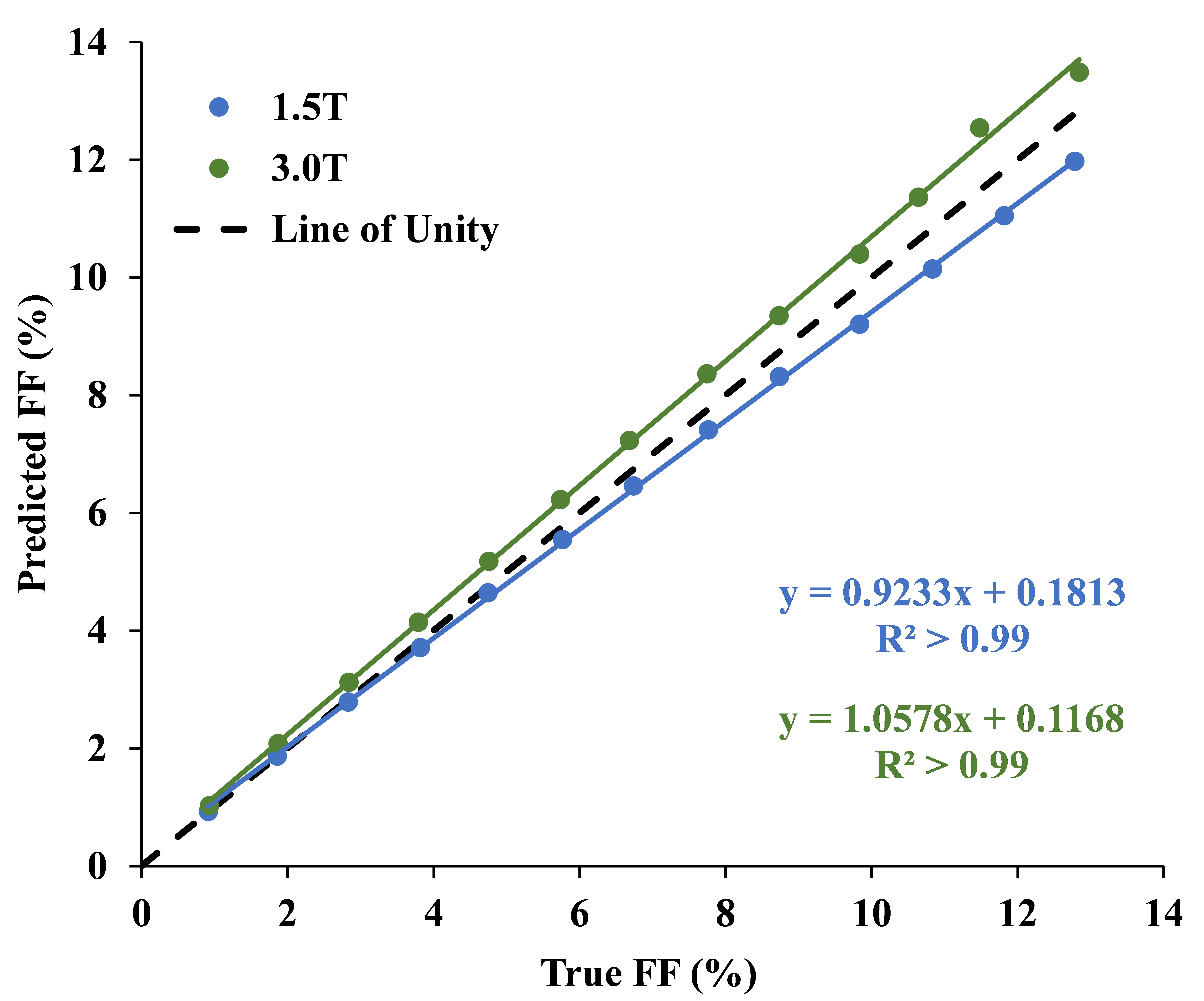
The FF of mice liver samples ranged from 0.05%–11.5%. Histograms of radii, NN distance, and regional anisotropy of FDs fitted with GDF for three representative liver samples with different FFs are shown in Figure 1. The virtual steatosis models were simulated with 0-13% FF, and they closely mimicked the in-vivo fat morphology in the actual histology image (Figure 2). As shown in Figure 3, for both field strengths, predicted R2* values showed positive correlation with FFs, with slopes similar to those of the in-vivo R2*-FF calibrations5 for χ=0.3ppm (P=0.06 for 1.5T; P=0.73 for 3.0T). χ=0.3ppm is in agreement with the magnetic susceptibility of fat measured in patients with steatosis.8 Figure 4 demonstrates that R2*F showed linearly increasing trend with FF similar to R2*W, and the mean R2*F-R2*W is 15.1s-1 at 1.5T and 30.3s-1 at 3.0T, similar to previous study by Hernando et al.9 The predicted FF values were also in excellent agreement with true FFs, with slopes ~1 (Figure 5). Hence, our simulations performed by creating realistic steatosis models and synthesizing MRI signal demonstrate that R2*W and R2*F are slightly different at low FFs as observed in in-vivo studies.10,11 However, at higher FFs R2*W and R2*F might show large differences and estimating independent R2* might produce accurate FFs. Also, considering independent R2* for water and fat might be important in co-existing conditions of iron overload as iron could affect the MRI signal of water and fat molecules differently due to their difference in molecular sizes.11 In these scenarios, R2*W and R2*F might be very different and estimating a weighted single R2* might introduce inaccuracies in both FF and R2* quantification, thereby causing bias in assessing steatosis and iron overload.Conclusion
Our study demonstrates the proof-of-concept for generating steatosis models from histologic data and synthesizing MRI signal to show the expected signal relaxation under conditions of steatosis.. Our results show that R2*W and R2*F are slightly different at low FFs and both demonstrate a positive correlation with FF with slopes of R2*W-FF similar to in-vivo calibrations. Future work involves simulating steatosis models at higher FFs and with iron overload.Acknowledgements
No acknowledgement found.References
1. Meisamy S, Hines CD, Hamilton G, et al. Quantification of hepatic steatosis with T1-independent, T2*-corrected MR imaging with spectral modeling of fat: blinded comparison with MR spectroscopy. Radiology. 2011;258(3):767-775.
2. Yu H, McKenzie CA, Shimakawa A, et al. Multiecho reconstruction for simultaneous water‐fat decomposition and T2* estimation. J Magn Reson Imaging. 2007;26(4):1153-1161.
3. Chebrolu VV, Hines CD, Yu H, et al. Independent estimation of T2* for water and fat for improved accuracy of fat quantification. Magn Reson Med. 2010;63(4):849-857.
4. Yamada I, Aung W, Himeno Y, Nakagawa T, Shibuya H. Diffusion coefficients in abdominal organs and hepatic lesions: evaluation with intravoxel incoherent motion echo-planar MR imaging. Radiology. 1999;210(3):617-623.
5. Bashir MR, Wolfson T, Gamst AC, et al. Hepatic R2* is more strongly associated with proton density fat fraction than histologic liver iron scores in patients with nonalcoholic fatty liver disease. J Magn Reson Imaging. 2019;49(5):1456-1466.
6. Hamilton G, Yokoo T, Bydder M, et al. In vivo characterization of the liver fat 1H MR spectrum. NMR Biomed. 2011;24(7):784-790.
7. Tipirneni‐Sajja A, Krafft AJ, Loeffler RB, et al. Autoregressive moving average modeling for hepatic iron quantification in the presence of fat. J Magn Reson Imaging. 2019;50(5):1620-1632.
8. Leporq B, Lambert SA, Ronot M, Vilgrain V, Van Beers B. Simultaneous MR quantification of hepatic fat content, fatty acid composition, transverse relaxation time and magnetic susceptibility for the diagnosis of non‐alcoholic steatohepatitis. NMR Biomed. 2017;30(10):e3766.
9. Hernando D, Liang ZP, Kellman P. Chemical shift–based water/fat separation: A comparison of signal models. Magn Reson Med. 2010;64(3):811-822.
10. Horng DE, Hernando D, Hines CD, Reeder SB. Comparison of R2* correction methods for accurate fat quantification in fatty liver. J Magn Reson Imaging. 2013;37(2):414-422.
11. Horng DE, Hernando D, Reeder SB. Quantification of liver fat in the presence of iron overload. J Magn Reson Imaging. 2017;45(2):428-439.
Figures