Introduction

We propose a magnetic resonance (MR) method to achieve high-resolution whole-brain low-frequency (LF) conductivity tensor imaging (CTI). Our methodology seeks to overcome the limitations of previous approaches - such as MR Electric Properties Tomography (MR-EPT) ¹ - by designing a framework independent from the Laplacian operator, which is noise sensitive and is less reliable at tissue boundaries. This objective is achieved by combining high frequency (HF) conductivity mapping based on water maps ² with multi-b-value diffusion tensor imaging (DTI) data ^3-5.

Methods

Theory
In what follows, HF refers to the Larmor frequency, whereas LF to the frequency range of the brain at rest ($$$\sim10Hz$$$). The LF conductivity tensor $$$\textbf{C}_{LF}$$$ is related to the extracellular water diffusion tensor $$$\textbf{D}_e$$$ according to ³:
$$\textbf{C}_{LF}= \frac{\chi_e \sigma_{HF}}{\chi_e d_e + (1-\chi_e) d_i \beta } \textbf{D}_e$$
where $$$\beta = 0.41$$$ ³, $$$\sigma_{HF}$$$ is the isotropic HF conductivity, $$$\chi_{e}$$$ the extracellular volume fraction, and $$$d_i$$$ and $$$d_e$$$ the intra- and extracellular water diffusivities.
Image Acquisition
Five healthy volunteers were scanned on a 3T Philips Ingenia scanner with a 32-channel receiver head coil. The acquisition protocol consists of:

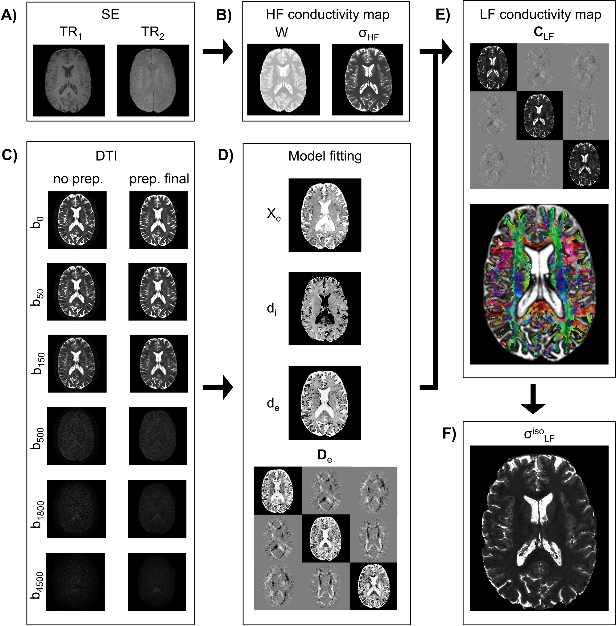
• a pair of 2D multi-slice spin echo (SE) T1w images acquired with in-plane isotropic resolution and slice thickness of 1mm. 81 slices were employed to cover the brain (slice gap 1mm). $$$TE$$$ was 11ms and flip angle / refocusing angles $$$90^o/180^o$$$. As in ², $$$TR_1$$$ and $$$TR_2$$$ were 700ms and 3000ms, respectively.
• DTI data acquired with an in-plane isotropic resolution and a slice thickness of 1.5mm. Slice gap was 1mm. 56 slices were acquired with multiband 2 ⁶. An in-plane SENSE factor of 2.5 was employed. Six b-vaues (Fig.1C) each with $$$n=16$$$ directions were acquired. Flip angle / refocusing angles were $$$90^o/180^o$$$, $$$TE=134ms$$$ and $$$TR=4899ms$$$.

Processing pipeline
To estimate $$$\sigma_{HF}$$$, the two SE images are fused to compute a water content map $$$W$$$ (Fig.1B). The latter is employed to calculate $$$\sigma_{HF}$$$ ² (note that this method does not rely on processing the phase of the $$$B1$$$ maps as in conventional MR-EPT techniques).
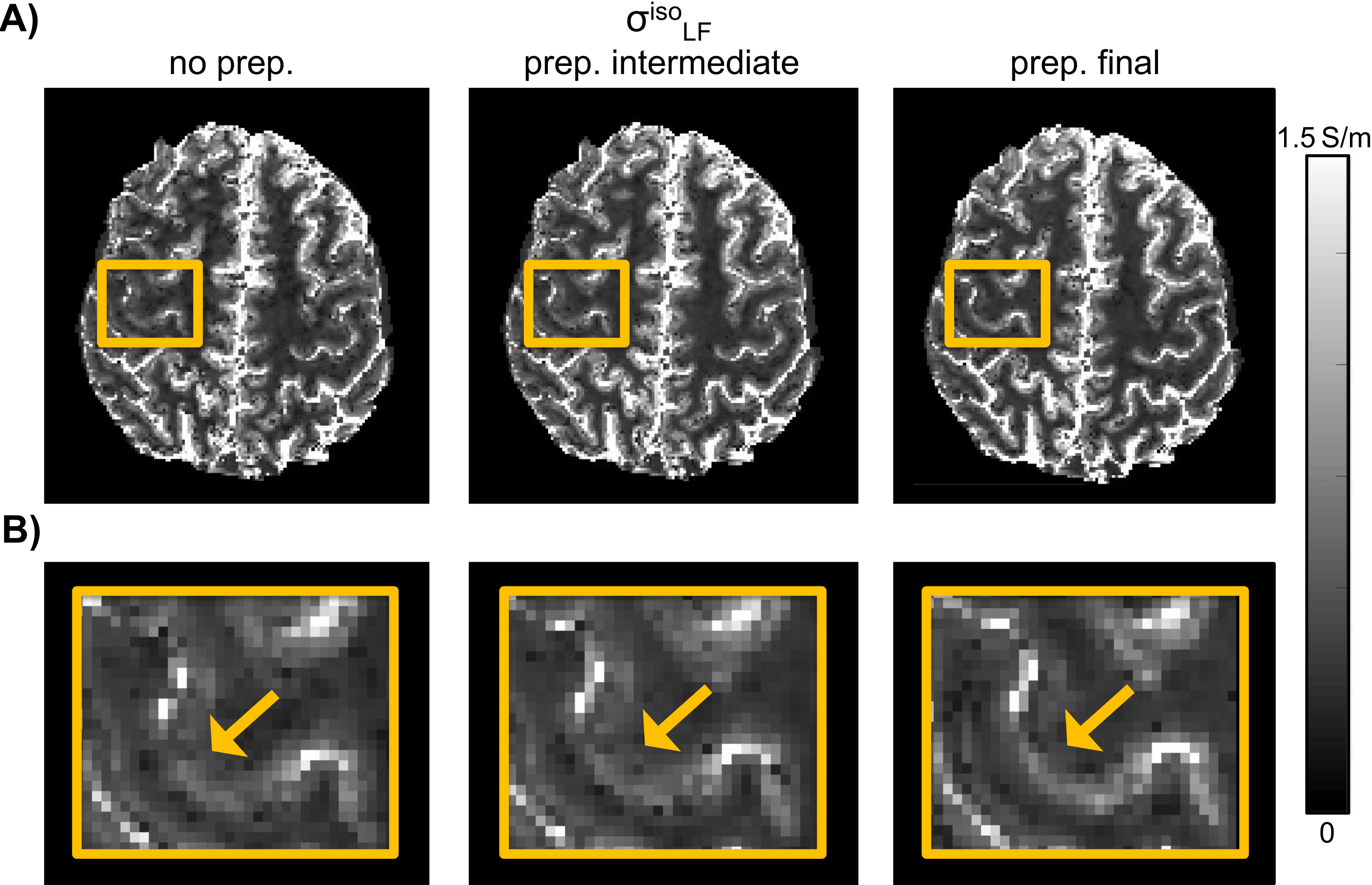
We preprocess the DTI according to an optimized pipeline (Fig.1C), which includes denoising ^7-8 plus bias field correction (prep. intermediate), together with distortion correction ⁹ plus rigid registration (prep. final).
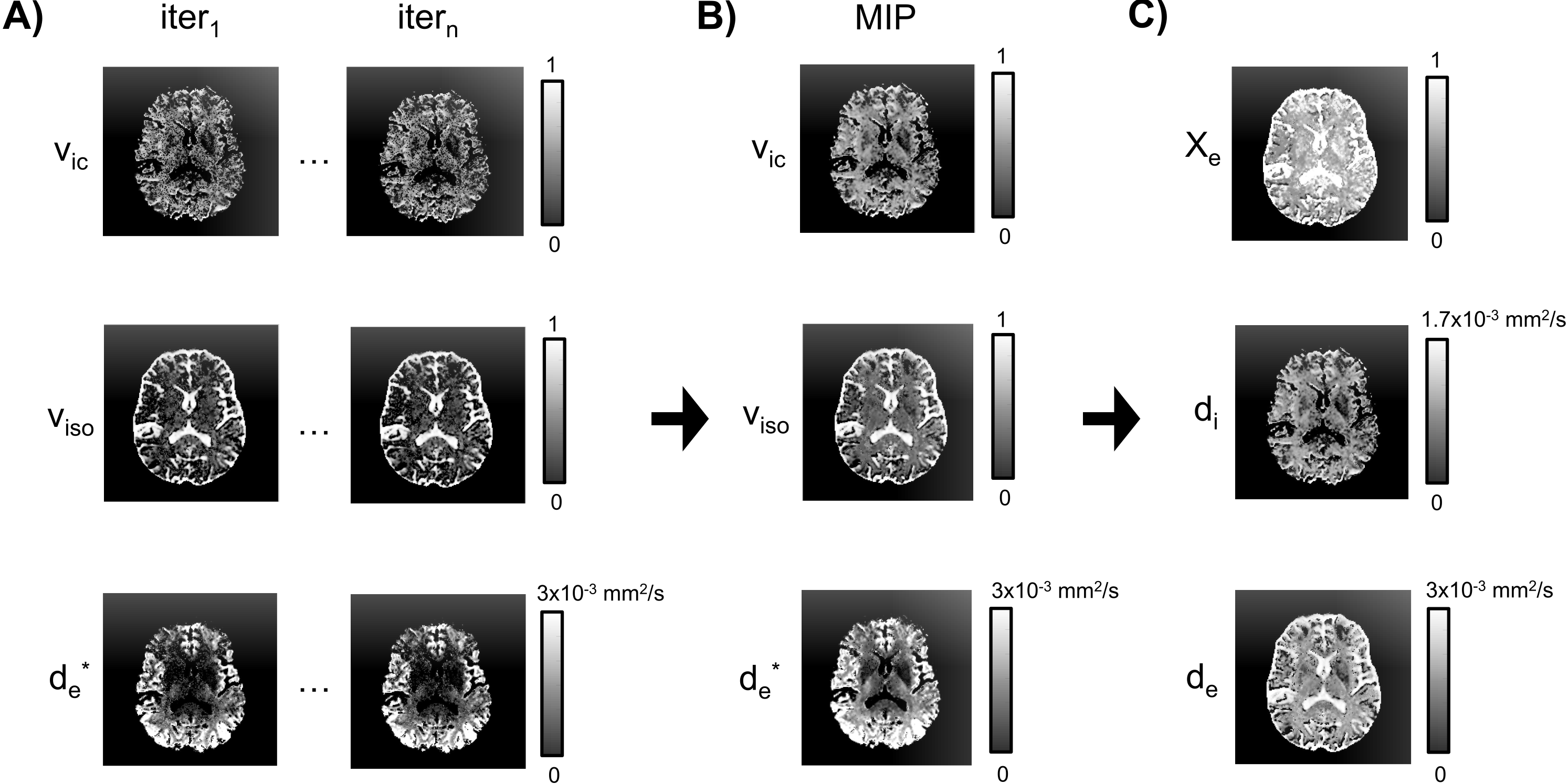
We estimate $$$\textbf{D}_e$$$, $$$\chi_{e}$$$, $$$d_i$$$, and $$$d_e$$$ (Fig.1D). To do so, we employ a NODDI-like ¹⁰ model, which depends on sub-variables $$$v_{ic}$$$, $$$v_{iso}$$$ and $$$d_e^*$$$ - respectively intracellular volume fraction, isotropic volume fraction and the extracellular mean diffusivity ⁴:
$$\frac{S_b}{S_o} = (1-v_{iso})(v_{ic}e^{-b v_{ic} d_{ic} }+(1-v_{ic})e^{-b (1-v_{ic})d_e^*})+v_{iso}e^{-b d_{iso}}$$
In this equation, $$$S_b$$$ is the DTI signal averaged over all gradient directions at each b-value $$$b$$$ and $$$S_o$$$ the signal without diffusion weighting applied. Note that in this model the intracellular diffusivity $$$d_{ic}$$$ and the isotropic water diffusivity $$$d_{iso}$$$ are set fixed from the literature ¹⁰ ($$$d_{ic}=1.7 \times 10^{-3} \frac{mm^2}{s}$$$ and $$$d_{iso}=3 \times 10^{-3} \frac{mm^2}{s}$$$).

Fig.2 reports details about the fitting. In order to improve the estimation of $$$v_{ic}$$$, $$$v_{iso}$$$ and $$$d_e^*$$$, several sub-fitting experiments are carried out. At each iteration (Fig.2A), a slightly different estimate for $$$S_b$$$ of equation 2 is employed, which is drawn by randomly choosing $$$n-1$$$ gradient directions from the $$$n=16$$$ available. The final estimates for $$$v_{ic}$$$, $$$v_{iso}$$$ and $$$d_e^*$$$ are computed by calculating the maximum intensity projection (MIP) maps across all iterations (Fig.2B). Once this is done, $$$\chi_e$$$, $$$d_e$$$ and $$$d_i$$$ (Fig2.C) are computed as ²:
$$\chi_e =(1-v_{iso})(1-v_{ic})+v_{iso}$$
$$d_e=\frac{(1-v_{iso})(1-v_{ic})^2 d_e^*}{\chi_e} + \frac{v_{iso} d_{iso}}{\chi_e}$$
$$d_i=v_{ic} d_{ic}$$
To compute $$$\mathbf{D}_e$$$ (Fig.1D, bottom), we estimate the diffusion tensor $$$\textbf{D}$$$ at $$$b=1000$$$ $$$\frac{s}{mm^2}$$$. Subsequently, we perform a singular value decomposition (SVD). By denoting with $$$d_{xx}$$$, $$$d_{yy}$$$ and $$$d_{zz}$$$ the eigenvalues ⁴:
$$\textbf{D}_e= \eta \textbf{D}$$
where
$$\eta = \frac{3 d_e}{d_{xx} + d_{yy} + d_{zz}}$$
Finally, all individual estimates are compounded together to form $$$\textbf{C}_{LF}$$$ (Fig.1E) by means of equation 1. An 'isotropic equivalent' LF conductivity map $$$\sigma_{LF}^{iso}$$$ (Fig.1F) is computed as:

$$\sigma_{LF}^{iso}=\sqrt[3]{c_{xx}c_{yy}c_{zz}}\qquad$$

where $$$c_{xx}$$$, $$$c_{yy}$$$ and $$$c_{zz}$$$ are the eigenvalues of a second SVD applied to $$$\textbf{C}_{LF}$$$.

Results

The estimation of $$$v_{ic}$$$, $$$v_{iso}$$$ and $$$d_e^*$$$ as a function of consecutive iterations of the fitting procedure (Fig.2A) plus their MIP combination (Fig.2B), led to stable estimates for $$$\chi_e$$$, $$$d_i$$$ and $$$d_e$$$ (Fig.2C).
The preprocessing applied to the diffusion data reduced the noise and improved spatial matching to the SE T1w data. Benefits include incremental improvements in the achieved spatial resolution for $$$\sigma_{LF}^{iso}$$$ with respect to no DTI preprocessing applied (no prep.) (see Fig.3A-B).
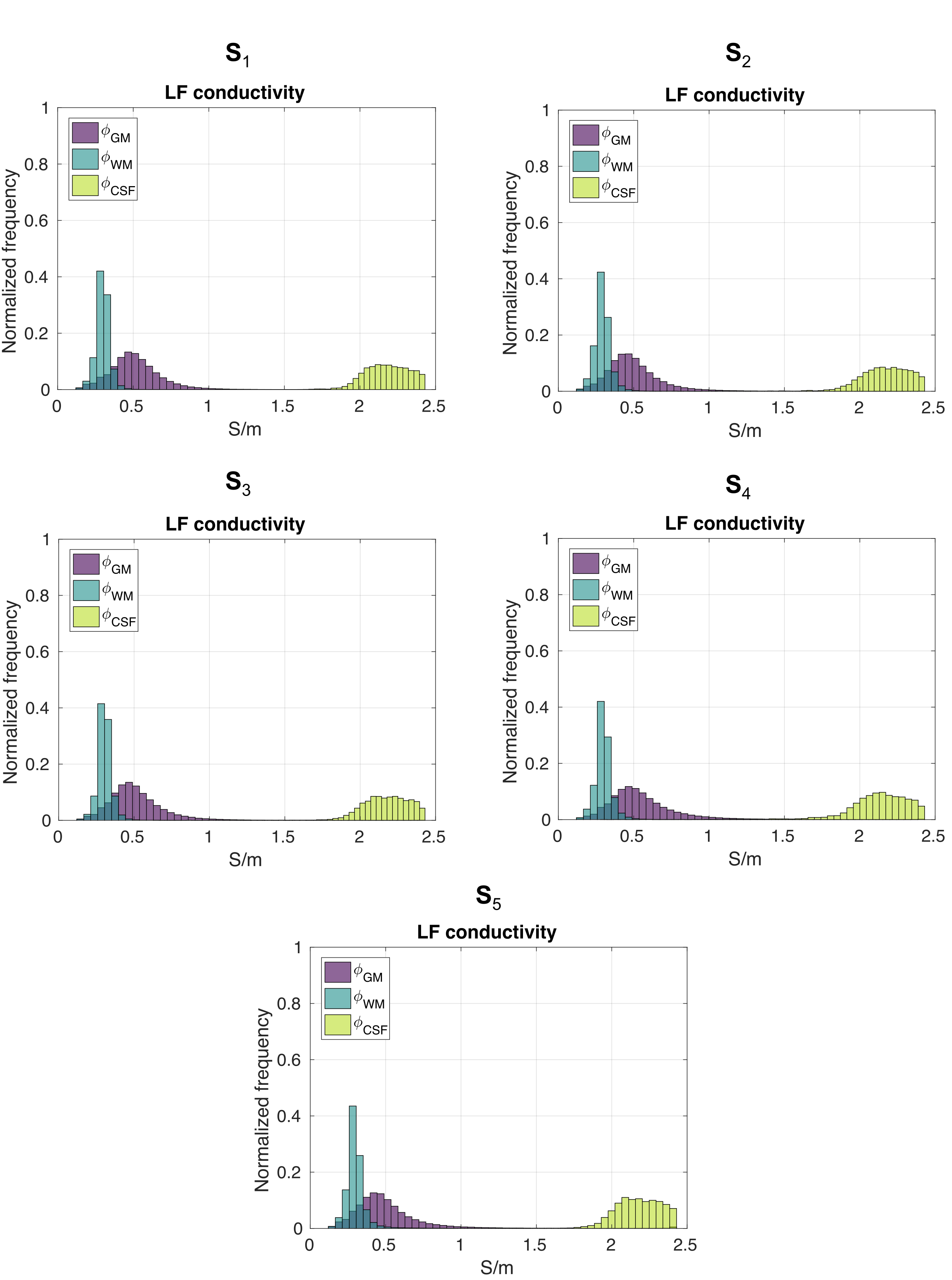
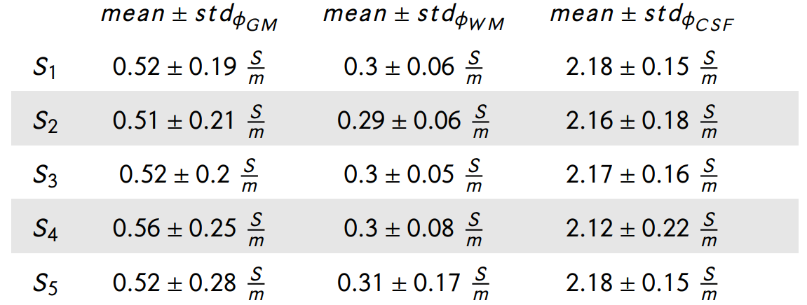
Normalized distributions $$$\phi$$$ for $$$\sigma_{LF}^{iso}$$$ of grey matter (GM), white matter (WM) and cerebrospinal fluid (CSF) are shown in Fig.4. Measured conductivity values are reported in Tab.1. Overall, our findings highlight noteworthy within- and between- subject variability of the conductivity values.

Conclusion and Discussion

In this study, a framework to achieve high-resolution whole-brain CTI mapping has been proposed. By optimizing $$$\textit{i}$$$) the pre-processing of the DTI data, and $$$\textit{ii}$$$) the fitting procedure, conductivity maps of excellent image quality can be produced. Our methodology does not require the use of a Laplacian operator as in conventional CTI methods ^3-5. This allows to retain spatial resolution and to improve the performances of the reconstruction at tissue boundaries. Consequently, partial volume effects are reduced leading to good discrimination of tissues with similar conductivity values, such as GM and WM.

Acknowledgements

The work was supported by the KU Leuven Special Research Fund (grant C16/15/070), the Research Foundation Flanders (FWO) (grants G0F76.16N, G0936.16N, EOS.30446199, I0050.18N, and postdoctoral fellowship 1211820N to MM) and the Italian Ministry of Health (Grant No. RF-2018-12366899). The authors would like to thank Luca Ghezzo for the support with MR data acquisition.