3786
Comparison of MR-based low-frequency electrical conductivity tensor using DT-MREIT and CTI: a biological tissue phantom study
Saurav Zaman Khan Sajib1, Munish Chauhan1, Sulagna Sahu1, Enock Boakye1, and Rosalind J Sadleir1
1School of Biological and Health Systems Engineering, Arizona State University, Tempe, AZ, United States
1School of Biological and Health Systems Engineering, Arizona State University, Tempe, AZ, United States
Synopsis
Diffusion tensor magnetic resonance electrical impedance tomography (DT-MREIT) and electrodeless conductivity tensor imaging (CTI) are two emerging modalities that can quantify low-frequency tissue anisotropic conductivity properties by considering the relationship between ion mobility and water diffusion. While both methods have potential applications to estimating neuro-modulation fields or formulating forward models used for electrical source imaging, a direct comparison of these two modalities has not yet been performed. Therefore, the aim of this study to test the equivalence of these two modalities.
INTRODUCTION
Magnetic Resonance Electrical Impedance Tomography (MREIT)1,2 has been developed to produce high-resolution isotropic low-frequency conductivity images from external-current-induced magnetic flux density $$$\left(B_z\right)$$$ data. Standard MREIT methods cannot be used for anisotropic imaging because of noise in measured data2. Kwon et al.3 developed the DT-MREIT technique to reconstruct conductivity distributions using $$$B_z$$$ and a priori anisotropic information contained in diffusion tensor $$$\left( \mathbf{\mbox{D}}\right)$$$ data4. However, both MREIT and DT-MREIT methods require an external current application, which may involve the risk of injury or peripheral neural stimulation. Sajib et al.5 later developed the electrodeless CTI method, which can provide both isotropic and anisotropic conductivity distributions6,7, by decomposing the high-frequency conductivity $$$\left(\sigma_H\right)$$$ measured using MR Electrical Properties Tomography8,9 (MREPT) into its extra- and intra-cellular parts and incorporating the tissue microstructure parameters estimated from multi-b-value diffusion-weighted images10-12. In the literature, both DT-MREIT3 and CTI5 methods have been used to determine the anisotropic conductivity distribution of in-vivo canine5,13 and human brains14,15. However, the equivalence of these two modalities has not yet been investigated. Therefore, this study aims to determine if low-frequency electrical tissue conductivity determined using MREIT, DT-MREIT, and CTI methods in a single biological tissue phantom are the same.METHODS
Phantom design: A cylindrical acrylic container with a diameter of 150 mm and a height of 140 mm was used to build the biological tissue phantom. Two opposing pairs of 50 x 50 mm2 carbon electrodes (HUREV, South Korea) were attached to the container perimeter. Three sections of bovine muscle, oriented in $$$x$$$ (left), $$$y$$$ (right), and $$$z$$$-directions (top) were then placed inside the chamber to provide anisotropic tissue properties (Fig-2c). An isotropic cylindrical conductive anomaly made of Tx-151 gel (diameter 40 mm, height 140 mm, conductivity 1.95 S/m at 10 Hz) was also placed at the bottom of the container. The phantom background was then filled with a 0.75 S/m (10 Hz) agarose gel.Imaging experiment: All MR data were measured using a 32-channel RF head coil in a 3.0T Phillips scanner (Phillips, Ingenia, Netherlands) located at the Barrow Neurological Institute (Phoenix, Arizona, USA). Table in Fig. 1(a) summarizes the imaging parameters used in this study. To match the dimension of the MREIT/MREPT data, the acquired DW-datasets were interpolated to $$$128\times128$$$ matrix size in subsequent data processing steps. A transcranial electrical stimulator (DC-STIMULATOR MR, neuroConn, Ilmenau, Germany) was used to deliver a 4.0 mA current through the two pairs of opposing electrodes $$$\left(\mathcal{E}=1,2\right)$$$. Fig.1(b)-(i) shows the measured MR data at the third-slice position.
Conductivity image reconstruction: In CTI-theory5, the low-frequency equivalent isotropic conductivity, $$$\sigma_L^{CTI}=\eta^{CTI}d_e^w$$$ and anisotropic conductivity tensor, $$$\mathbf{\mbox{C}}^{CTI} =\eta^{CTI} \mathbf{\mbox{D}}_e^w$$$ is estimated from the extra-cellular water self-diffusivity, $$$d_e^w$$$ and diffusion tensor $$$ \mathbf{\mbox{D}}_e^w$$$. The scale-factor is expressed as5
$$\eta^{CTI}=\frac{\alpha\sigma_H}{\alpha d_e^w+\beta(1-\alpha)d_i^w}\quad\quad\quad\quad\quad\quad\mbox{(1)}$$
where, $$$1-\alpha,~d_i^w$$$ denotes the intra-cellular space volume fraction and water diffusivity, respectively, and $$$\beta$$$ is the intra-to-extra-cellular ion concentration ratio. A convection-reaction based partial-differential-equation (PDE) was solved to obtain the from the measured B1-phase data (crEPT)9. The $$$L^2$$$-norm of a multi-compartment model6 of the observed multi-b-value-DW data was minimized at each pixel position to find the microstructure parameters, $$$\left(\alpha,~d_e^w,~d_i^w\right)$$$6. The $$$d_e^w$$$ and the eigenvalues of the $$$\mathbf{\mbox{D}}$$$ found at b=700 sec/mm2 was then used to estimate the $$$\mathbf{\mbox{D}}_e^w$$$.6
Using the estimated projected current density16 $$$\mathbf{\mbox{J}}^{P,\mathcal{E}}, \mathcal{E}=1,2$$$ from current applications we also determined the effective isotropic conductivity17 $$$\left(\sigma_L^{EIT}\right)$$$ and conductivity tensor3 $$$\left(\mathbf{\mbox{C}}^{EIT}=\eta^{EIT}\mathbf{\mbox{D}}_e^w\right)$$$. To reconstruct the $$$\sigma_L^{EIT},~\mbox{or}~\eta^{EIT}$$$ we must solve a two-dimensional Poisson’s equation with a known boundary value18. Without prior knowledge of the phantom boundary conductivity or scale-factor values, either the MREIT or DT-MREIT methods provide only ‘apparent’ conductivity contrasts. Since the CTI method is expected to provide the absolute conductivity, in this study we assigned the boundary conductivity to be that obtained from CTI reconstructions.
RESULTS and DISCUSSION
To obtain a stable numerical solution in crEPT, a scaled artificial diffusion term must be added6. Fig. 2(a) shows the $$$\sigma_H$$$ image reconstructed with an artificial diffusion term coefficient of 0.05. The estimated $$$d_e^w,~d_i^w,~\alpha$$$ images obtained from multi-b-value DW-data are shown in Fig. 2(b)-(d), respectively. The reconstructed $$$|\mathbf{\mbox{J}}^{P,\mathcal{E}}|,\mathcal{E}=1,2$$$ images are also displayed in Fig. 2(e)-(f).For CTI image reconstruction we set the unknown $$$\beta$$$-value at 1.0. The reconstructed scale-factor obtained using CTI ($$$\beta=1$$$) or DT-MREIT data are displayed in Fig. 3(a) and (e) respectively. The scale-factors were then multiplied with $$$\mathbf{\mbox{D}}_e^w$$$ to obtain the corresponding conductivity tensors. To compare anisotropic properties, we decomposed the reconstructed $$$\mathbf{\mbox{C}}\left(\mathbf{\mbox{C}}^{CTI}/\mathbf{\mbox{C}}^{EIT}\right)$$$ into longitudinal $$$\left(\lambda^C_{\parallel}=\lambda^C_1\right)$$$ and transversal $$$\left(\lambda_{\bot}^C=\frac {\lambda_2^C+\lambda_3^C} {2} \right)$$$ directions, where $$$\lambda_1^C\geq\lambda_2^C\geq\lambda_3^C$$$ are the three eigenvalues. Fig. 3(b)-(c) and (f)-(g) shows the reconstructed longitudinal and transverse conductivities obtained using the CTI and DT-MREIT methods. The effective isotropic conductivity obtained from the methods are also shown in Fig. 3(d) and (h), respectively. The reconstructed conductivity values in agar, muscle, and Tx-151 region is compared in Fig. 4. The plot in Fig. 5 shows how reconstructed CTI conductivities varied as a function of $$$\beta$$$. As anticipated, the conductivity reconstructed in muscle regions varied with $$$\beta$$$. However, conductivity in other regions did not depend on $$$\beta$$$ .
CONCLUSIONS
Using a biological tissue phantom data we have demonstrated that the CTI, DT-MREIT and MREIT method may provide equivalent tissue conductivity.Acknowledgements
This work was supported by award RF1MH114290 to RJS.References
- Seo J K and Woo E J. Electrical tissue property imaging at low frequency using MREIT. IEEE Trans. Biomed. Eng. 2014; 61(5): 1390-99.
- Seo J K and Woo E J. Magnetic resonance electrical impedance tomography. SIAM Rev. 2011;53(1):40-68.
- Kwon O I, Jeong W C and Sajib S Z K et al. Anisotropic conductivity tensor imaging in MREIT using directional diffusion rate of water molecules. Phys. Med. Biol. 2014; 59 (12): 2955-74.
- Tuch D S, Wedeen V J and Dale A M et al. Conductivity tensor mapping of the human brain using
diffusion tensor MRI. Proc. Nat. Acad. Sci. 2001; 98(20): 11697-701.
- Sajib S Z K, Kwon O I and Kim H J et al. Electrodeless conductivity tensor imaging (CTI) using MRI: basic theory and animal experiments. Biomed. Eng. Lett. 2018; 8(3): 273-82.
- Lee M B, Jahng GH and Kim H J et al. Extracellular electrical conductivity property imaging by decomposition of high-frequency conductivity at Larmor-frequency using multi-b-value diffusion-weighted imaging. PLos One. 2020; 15(4): e0230903.
- Jahng GH, Lee M B and Kim H J et al. Low-frequency dominant electrical conductivity imaging of in-vivo human brain using high-frequency conductivity at Larmor-frequency and spherical mean diffusivity without external current injection. NeuroImage. 2021; 225: 117466.
- Seo J K, Kim D H, and Lee J et al. Electrical tissue property imaging using MRI at dc and Larmor frequency. Inverse Problems. 2012; 28(8):084002.
- Gurler N and Ider Y Z. Gradient-based electrical conductivity imaging using MR phase. Magn. Reson. Med. 2017; 77(1): 137-50.
- Tanner J E. Self-diffusion of water in frog muscle. Biophys. J. 1979; 28(1): 107-16.
- Gelderen P V, Despres D, and vanZIJL P C M et al. Evaluation of restricted diffusion in cylinders. Phosphocreatine in rabbit leg muscle. Journal Magn. Reson. Series B. 1994; 103(3): 255-60.
- Stanisz G J, Szafer A, Wright G A
et al. An analytical model of restricted diffusion in bovine optic nerve. Magn
Reson. Med. 1997; 37(1): 103-11.
- Jeong W C, Sajib S Z K and Katoch N. et al. Anisotropic conductivity tensor imaging of in vivo canine brain using DT-MREIT. IEEE Trans. Med. Imag. 2017;36(1):124-31.
- Chauhan M., Indahlastari A. and Kasinadhuni A K et al. Low-frequency conductivity tensor imaging of human head in vivo using DT-MREIT: first study. IEEE Trans. Med. Imag. 2018;37(4):966-76.
- Katoch N, Choi B K, and Sajib S Z K et al. Conductivity tensor imaging of in vivo human brain and experimental validation using giant vesicle suspension. IEEE Trans. Med. Imaging. 2019; 38(7):1569-77.
- Park C, Lee BI, and Kwon O I. Analysis of recoverable current from one component of magnetic flux density in MREIT. Phys. Med. Biol. 2007; 52(11):3001-13.
- Nam H S, Park C, and Kwon O I. Non-iterative conductivity reconstruction algorithm using projected current density in MREIT. Phys. Med. Biol. 2008;53(23):6947-61.
- Sajib S Z K, Katoch N, and Kim H J et al. Software toolbox for low-frequency conductivity and current density imaging using MRI. IEEE Trans. Biomed. Eng. 2017; 64(11):2505-14.
- Kwon O I, Jeong W C, and Sajib S Z K et al. Reconstruction of dual-frequency conductivity by optimization of phase map in MREIT and MREPT. BioMed Eng. OnLine. 2014; 13:1-15.
- Oh T I, Jeong W C, and Kim J E et al. Noise analysis in fast magnetic resonance electrical impedance tomography (MREIT) based on spoiled multi gradient echo (SPMGE) pulse sequence. Phys. Med. Biol. 2014; 59 (2014): 4723-38.
Figures
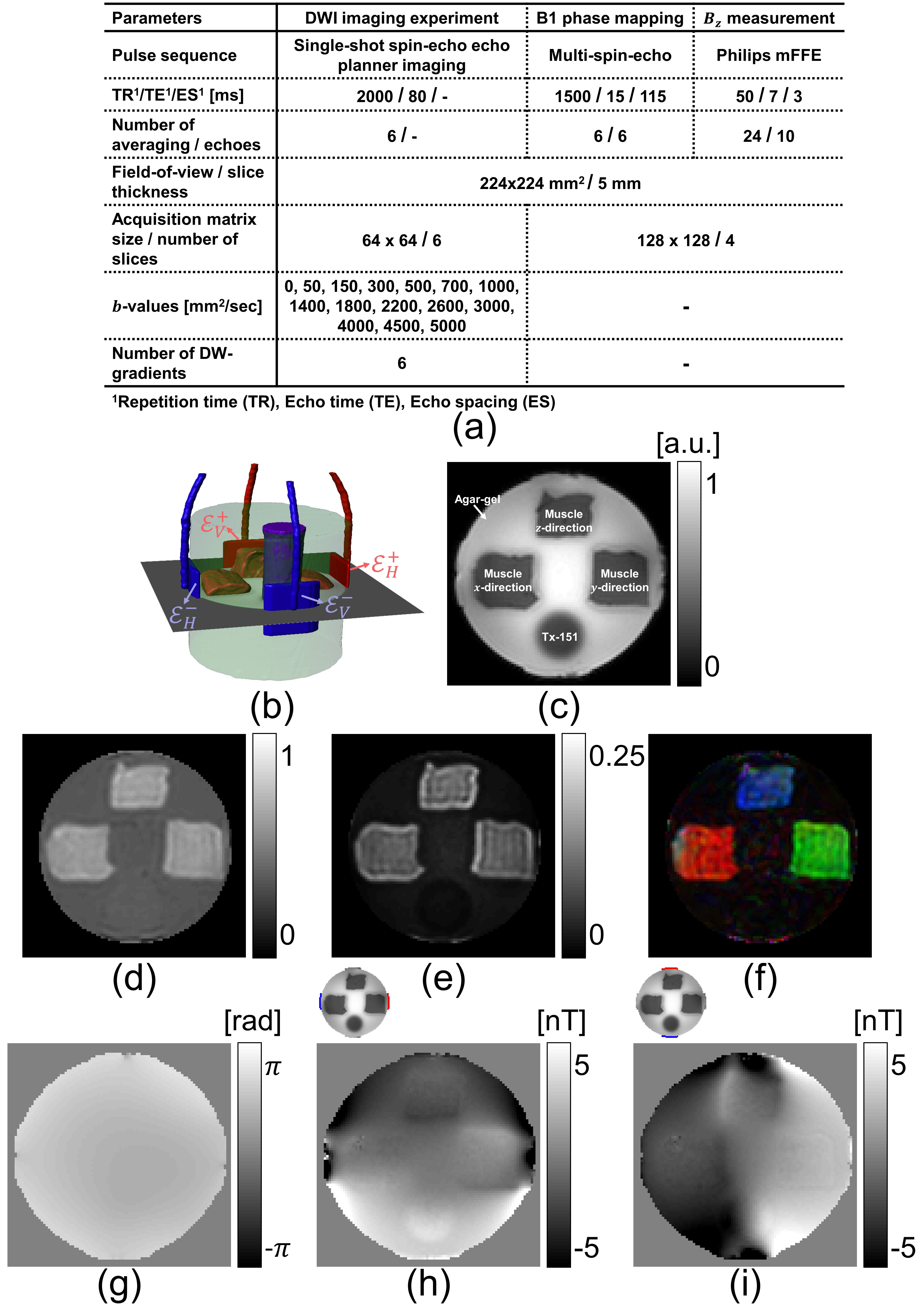
Figure
1: (a)
Imaging experiment parameters. (b) Computational model geometry of the phantom
with attached electrodes and wire tracks. (c) MR magnitude image of the third
slice acquired during MREIT experiment. Direction combined normalized DW-MR
images at b-value (d) 500 (e) 2600 sec/mm2. (f) Color-coded
fractional anisotropic map calculated from b=700 sec/mm2. (g)
Echo-combined18 B1-phase image. Current induced optimized19 $$$B_z$$$ flowing through the (h)
horizontal and (i) vertical electrode pairs.
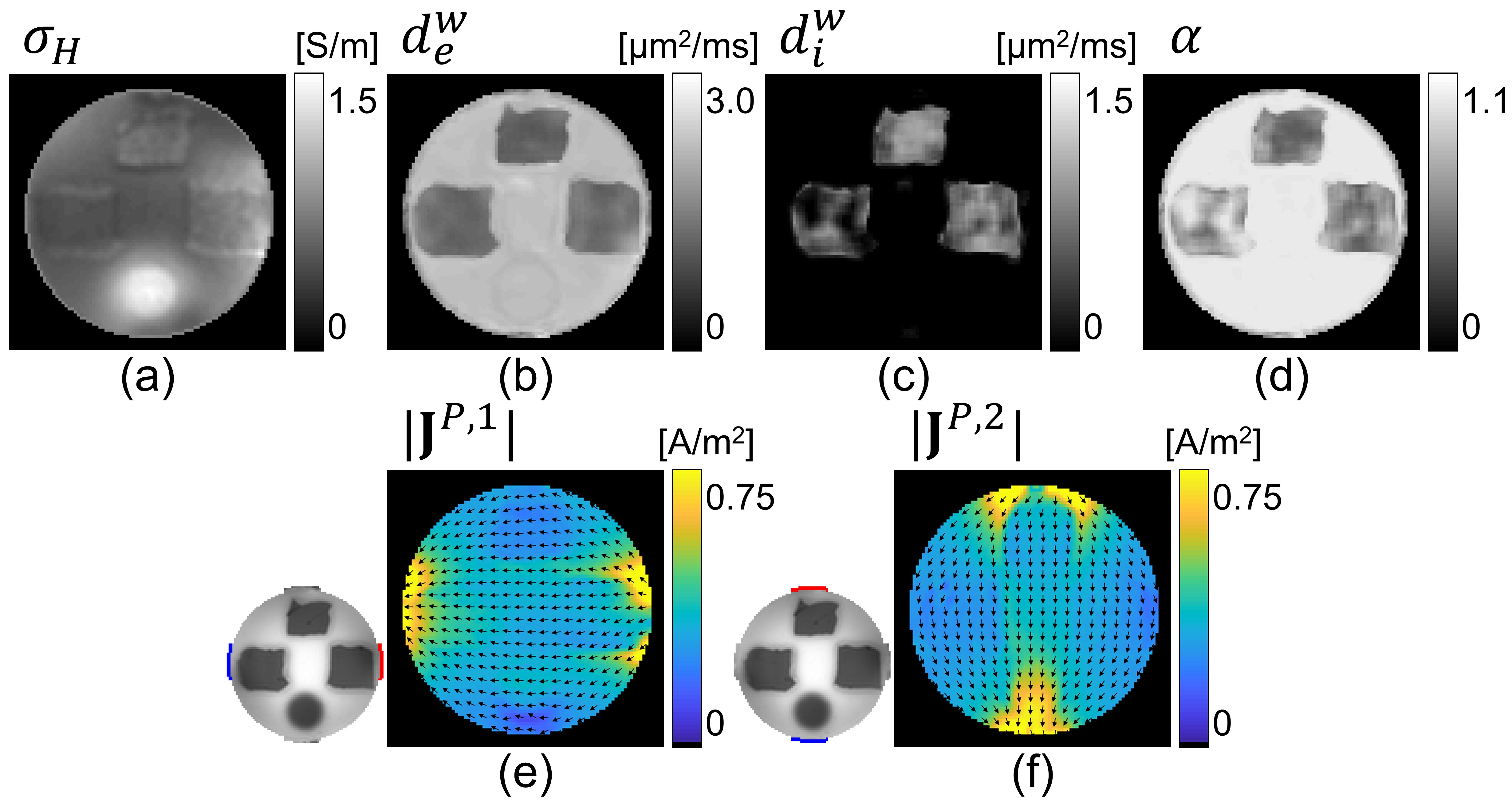
Figure 2: (a)
Reconstructed high-frequency conductivity $$$\left(\sigma_H\right)$$$ found using MREPT method at 128 MHz. Extra-, intra-cellular water diffusion and
extra-cellular volume fraction maps are shown in (b), (c), and (d), respectively.
Reconstructed $$$|\mathbf{J}^P|$$$ images
for (e) horizontal and (f) vertical electrode pairs. Normalized arrow-vectors
show the direction of the current flow.
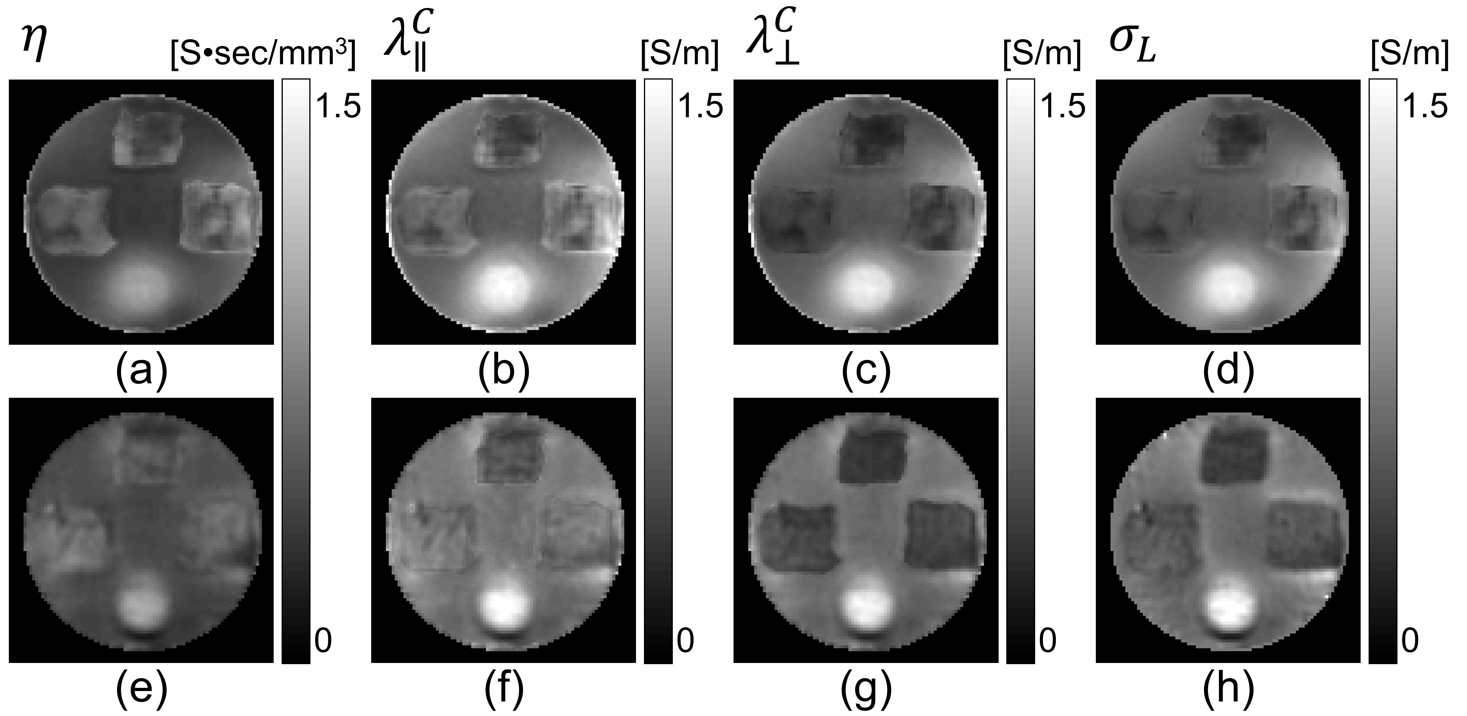
Figure 3: (a)
Reconstructed scale factor images obtained from CTI with
(b) Scale factors found using DT-MREIT method.
The longitudinal and transversal components of the conductivity tensors are
displayed in (b)-(c) for CTI and (f)-(g) for the DT-MREIT method. The
low-frequency equivalent isotropic conductivity obtained from the CTI and MREIT
method are shown in (d) and (h), respectively.
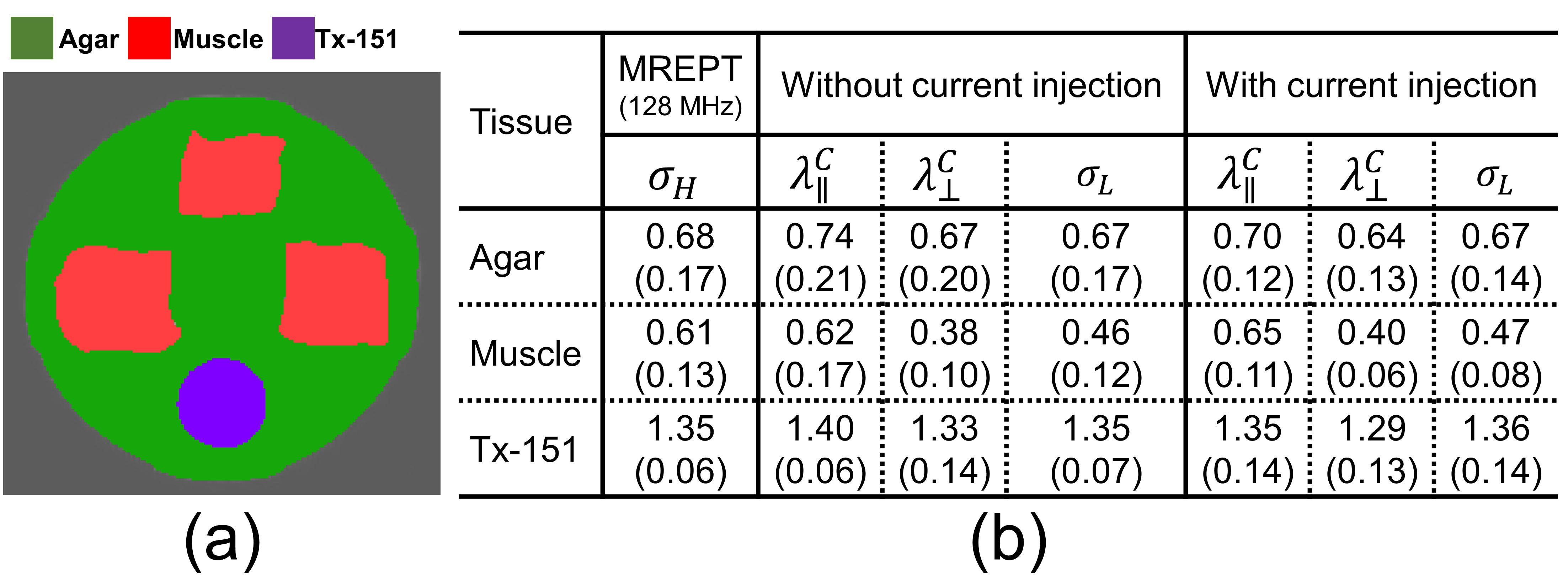
Figure 4: (a)
Segmented tissue mask used to compare conductivity values in the table shown in
(b). (b) Table compares the numerical values of the tissues obtained from the
MREPT, MREIT, DT-MREIT, CTI, methods for the reconstructed data shown in Fig. 3.
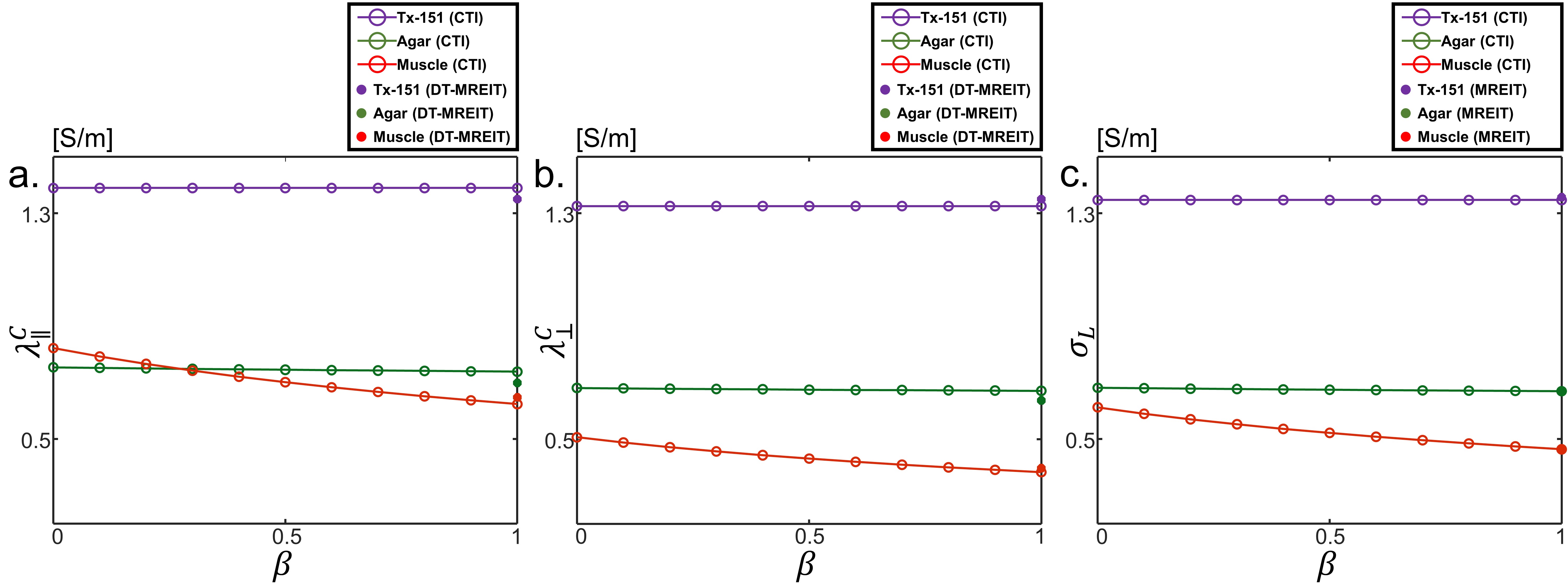
Figure 5: Variation
of the reconstructed conductivity found using CTI or DT-MREIT using different values
of $$$\beta$$$.