3783
An Application of a Projected Newton Method to Electrical Properties Estimation via Global Maxwell Tomography
Jose EC Serralles1, Ilias I Giannakopoulos2, Jacob K White1, Luca Daniel1, and Riccardo Lattanzi2,3,4
1Electrical Engineering and Computer Science, Computational Prototyping Group (CPG), Research Laboratory of Electronics (RLE), Department of Electrical Engineering and Computer Science (EECS), Massachusetts Institute of Technology (MIT), Cambridge, MA, United States, 2Center for Advanced Imaging Innovation and Research (CAI2R), Department of Radiology, New York University Grossman School of Medicine, New York, NY, United States, 3The Bernard and Irene Schwartz Center for Biomedical Imaging (CBI), Department of Radiology, New York University Grossman School of Medicine, New York, NY, United States, 4Vilcek Institute of Graduate Biomedical Sciences, New York University Grossman School of Medicine, New York, NY, United States
1Electrical Engineering and Computer Science, Computational Prototyping Group (CPG), Research Laboratory of Electronics (RLE), Department of Electrical Engineering and Computer Science (EECS), Massachusetts Institute of Technology (MIT), Cambridge, MA, United States, 2Center for Advanced Imaging Innovation and Research (CAI2R), Department of Radiology, New York University Grossman School of Medicine, New York, NY, United States, 3The Bernard and Irene Schwartz Center for Biomedical Imaging (CBI), Department of Radiology, New York University Grossman School of Medicine, New York, NY, United States, 4Vilcek Institute of Graduate Biomedical Sciences, New York University Grossman School of Medicine, New York, NY, United States
Synopsis
Global Maxwell Tomography (GMT) is a recently introduced technique that estimates tissue electrical properties from magnetic resonance measurements by solving an inverse scattering problem. In this work, we propose a new implementation of GMT that uses a Projected Newton method to minimize the cost function, instead of the quasi-Newton method employed by the original GMT. We demonstrated the new approach with two numerical experiments, using a four--compartment phantom and a realistic head model. Compared to the results obtained with the original GMT, the number of iterations required for convergence was drastically reduced and the estimated EP were more accurate.
Introduction
Global Maxwell Tomography (GMT) is a recently introduced volume-integral-equation-based method for non-invasive estimation of tissue electrical properties (EP), namely electric permittivity and conductivity, from magnetic resonance (MR) measurements [1,2]. GMT is posed as a volumetric inverse problem with respect to the EP. The cost function of GMT is minimized using L-BFGS-B, or L-BFGS with box constraints [3], a quasi-Newton algorithm that forms approximations of the Hessian. Initial numerical experiments with a human-head phantom showed an average error in the estimated permittivity and conductivity of 3.82% and 2.33%, respectively, after 1000 iterations, starting from a homogeneous initial guess. In this work, we present a new implementation of GMT that relies on the Projected Newton algorithm [4], with the goal of improving the accuracy of the EP reconstructions, while reducing the number of iterations.Theory
We modified the original cost function of GMT [1,2] by removing a square-root. Furthermore, in the proposed implementation we operate over the pointwise fields which means that the magnetic and electric fields are multiplied by the inverse of the Grammian $$$\mathbf{\Delta}$$$:$$\mathbf{h}_t=\mathbf{h}_i+\mathbf{\Delta}^{-1}\mathbf{K}\mathbf{J}\text{, and}$$
$$\mathbf{A}(\mathbf{\epsilon})\mathbf{J}=\left(\mathbf{I}-\mathbf{\Delta}^{-1}\mathbf{P}(\tfrac{\chi}{\epsilon})\mathbf{N}\right)\mathbf{J}=c_e\mathbf{P}(\tfrac{\chi}{\epsilon})\mathbf{e}_i$$
We solve the following optimization problem:
$$\min_{\epsilon\in\mathbb{C}^N}f(\epsilon)+\alpha{f_r(\epsilon)}\ \text{s.t.}\ \rm{Re}(\epsilon)\geq{1}\ \&\ \rm{Im}(\epsilon)\leq{0}\text{,}$$
where $$$f(\epsilon)$$$ is the data mismatch cost function and $$$f_r(\epsilon)$$$ is the Match Regularization cost function.
The data mismatch cost function operates over estimated and measured (with the hat) $$$\mathbf{b}_1^+$$$:
$$f\!\left(\mathbf{\epsilon},\mathbf{\overline{\epsilon}}\right)=\sum_k\sum_n\|\mathbf{\delta}_{kn}\|_2^2=\sum_k\sum_n\|\mathbf{b}_k\odot\overline{\mathbf{b}_n}-\hat{\mathbf{b}}_k\odot\overline{\hat{\mathbf{b}}_n}\|_2^2$$
where $$$\odot$$$ is the Hadamard product. The two summations in $$$n$$$ and $$$k$$$ iterate over all of the unique field maps of a multiple-channel transmit array. The gradient of the cost function in the CR-calculus sense is given by
$$\left(\frac{\partial f}{\partial\mathbf{\epsilon}}\right)^\ast=\left[\sum_k\mathbf{Q}^{\rm{T}}\!\left(\overline{\mathbf{\psi}_k}\odot\gamma_k\right)\right]\oslash\overline{\mathbf{\epsilon}}^2\text{,}$$
where
$$\mathbf{\psi}_k=\mathbf{\Delta}^{-1}\mathbf{N}\mathbf{J}_k+c_e\mathbf{e}_k^i$$
$$\mathbf{\gamma}_k=\mathbf{\Omega}^{\ast}\left(\sum_n\mathbf{b}_n\odot\mathbf{\delta}_{kn}\right)$$
$$\mathbf{\Omega}=\mu_0\mathbf{F}\mathbf{\Delta}^{-1}\mathbf{K}\mathbf{A}^{-1}\text{.}$$
In order to apply Newton to Global Maxwell Tomography, we require the second derivatives in the CR-calculus sense:
$$\frac{\partial}{\partial{\epsilon}}\frac{\partial f}{\partial\mathbf{\epsilon}}^\ast=\rm{D}^{-2}(\overline{\mathbf{\epsilon}})\mathbf{Q}^{\rm{T}}\sum_k\rm{D}(\overline{\mathbf{\psi}_k})\mathbf{\Omega}^{\ast}\!\left(\sum_n\rm{D}(\mathbf{\delta}_{kn})\mathbf{\Omega}\rm{D}(\mathbf{\psi}_n)+\rm{D}\left(|\mathbf{b}_n|^2\right)\mathbf{\Omega}\rm{D}(\mathbf{\psi}_k)\right)\mathbf{Q}\rm{D}^{-2}(\mathbf{\epsilon})$$
$$ \begin{split}\frac{\partial}{\partial\overline{\mathbf{\epsilon}}}\frac{\partial{f}}{\partial\mathbf{\epsilon}}^\ast= &-2\rm{D}^{-3}(\overline{\mathbf{\epsilon}})\rm{D}\!\left(\sum_k\mathbf{Q}^{\rm{T}}\!\left(\overline{\mathbf{\psi}_k}\odot\gamma_k\right)\right)\\&+\rm{D}^{-2}(\overline{\mathbf{\epsilon}})\sum_k\mathbf{Q}^{\rm{T}}\rm{D}(\overline{\mathbf{\psi}_k})\mathbf{A}^{-\ast}\!\left[\mathbf{N}^{\ast}\rm{D}(\mathbf{\gamma}_k)+\mu_0\mathbf{K}^{\ast}\mathbf{F}^{\ast}\rm{D}(\mathbf{b}_k)\sum_n\rm{D}(\mathbf{b}_n)\overline{\mathbf{\Omega}}\rm{D}(\overline{\mathbf{\psi}_n})\right]\mathbf{Q}\rm{D}^{-2}(\overline{\mathbf{\epsilon}})\\&+\rm{D}^{-2}(\overline{\mathbf{\epsilon}})\sum_k\mathbf{Q}^{\rm{T}}\rm{D}(\mathbf{\gamma}_k)\mathbf{\Omega}^{\rm{T}}\!\left[\sum_n\rm{D}(\overline{\mathbf{\delta}_{kn}})\overline{\mathbf{\Omega}}\rm{D}(\overline{\mathbf{\psi}_n})+\rm{D}\left(|\mathbf{b}_n|^2\right)\overline{\mathbf{\Omega}}\rm{D}(\overline{\mathbf{\psi}_k})\right]\mathbf{Q}\rm{D}^{-2}(\overline{\mathbf{\epsilon}})\end{split}
$$
When it comes to the Hessian matrix-vector product, we treat the Hessian as a real-valued matrix $$$\mathbf{H}\in\mathbb{R}^{2N\times2N}$$$. In order to switch between real- and complex-valued vectors, we define the operator $$$\mathbf{R}\colon\mathbb{C}^{N}\to\mathbb{R}^{2N}$$$ that concatenates the real and imaginary parts of the input and its inverse $$$\mathbf{R}^{-1}\colon\mathbb{R}^{2N}\to\mathbb{C}^{N}$$$. The Hessian matrix-vector product $$$\mathbf{H}\mathbf{v}$$$ is given by
$$\mathbf{H}(\epsilon)\mathbf{v}=\mathbf{R}\!\left( \frac{\partial}{\partial{\epsilon}}\frac{\partial f}{\partial\mathbf{\epsilon}}^\ast z +\frac{\partial}{\overline{\partial{\epsilon}}}\frac{\partial f}{\partial\mathbf{\epsilon}}^\ast\overline{z}\right)\text{,}$$
where $$$z=\mathbf{R}^{-1}\!\left(v\right)$$$.
Methods
We used the Magnetic Resonance Integral Equation (MARIE) simulation tool [5] for the forward problem of GMT, employing the piecewise linear basis functions for the volumetric currents [6]. Additionally, as in the original GMT publication [1], we neglected the coupling between the head and the incident fields, which is expected to have a negligible effect.We used Projected Newton [4] as the optimizer when estimating the electrical properties. Projected Newton is a modification of Newton's Method that allows for bound constraints on the decision variables. In addition, when solving for the Newton step $$$\mathbf{H}\mathbf{\Delta}\mathbf{\epsilon}=-\mathbf{g}(\mathbf{\epsilon})$$$, we used the minres algorithm for a loose tolerance of $$$10^{-1}$$$ and a maximum of 7 iterations because the Hessian is not positive semi-definite.
We performed numerical experiments on the same four-compartment tissue-mimicking phantom (4,096 voxels at a 6 mm isotropic resolution) and realistic "Billie" head model [7] (25,575 voxels at a 5 mm isotropic resolution) used in previous work [1], with the same parameters for the regularizer (Figure 1). We used $$$8$$$ idealized excitations [1] as incident fields, with a peak SNR of 50 and 200 for the four-compartment and head phantom, respectively. The operating frequency and the electrical properties were set for $$$B_0 = 7$$$Tesla.
Results
Figure 2 compares the initial and final EP estimates with the ground truth, for the four-compartment phantom. Starting from a homogeneous initial guess of EP, GMT converged in 74 iterations. The mean errors were 0.27% and 0.48% for $$$\epsilon_{\rm{R}}$$$ and $$$\sigma$$$, respectively. The maximum errors were 1.05% and 1.72% for $$$\epsilon_{\rm{R}}$$$ and $$$\sigma$$$, respectively.For the head phantom, starting again from a worst–case homogeneous guess, GMT converged after 103 iterations. The mean errors were 4.5% and 3% for $$$\epsilon_{\rm{R}}$$$ and $$$\sigma$$$, respectively. The maximum errors were 98.6% and 97.7% for $$$\epsilon_{\rm{R}}$$$ and $$$\sigma$$$, respectively. These peak errors were due to one-off voxels in regions of very high contrast, as suggested by Figure 3.
Discussion & Conclusion
We demonstrated a new implementation of GMT that uses a Projected Newton method as the optimizer. Similar results to the original GMT, based on L-BFGS-B method, were obtained in considerably fewer iterations. For the 4-compartment phantom, we saw a reduction in iterations by roughly a factor of two. For the realistic head phantom, the Projected Newton approach converged in 103 iterations, yielding results with comparable mean errors to 1000 L-BFGS-B iterations. The peak errors were considerably lower with Projected Newton: 98.6% vs. 262% for $$$\mathbf{\epsilon}_{\rm{R}}$$$. Additionally, the errors in our new approach were due to one-off voxels, whereas previously the large errors in estimated EP were artifacts that did not correspond to any tissue values. Therefore, for complex geometries, Projected Newton not only drastically reduces the number of iterations, but also yields more accurate and artifact-free solutions. Future work on GMT will try to address one-off errors in regions of extremely high contrast using more sophisticated regularization and Machine Learning methods. In conclusion, this work shows that the application of Projected Newton further cements GMT as one of the most accurate MR-based EP estimation algorithms implemented to date.Acknowledgements
This work was supported by NIH R01 EB024536 and by NSF 1453675. It was performed under the rubric of the Center for Advanced Imaging Innovation and Research (CAI$$$^2$$$R, www.cai2r.net), an NIBIB Biomedical Technology Resource Center (NIH P41 EB017183).References
- Serrallés, J. E. C., Giannakopoulos, I. I., Zhang, B., Ianniello, C., Cloos, M. A., Polimeridis, A. G., ... \& Lattanzi, R. (2019). Noninvasive estimation of electrical properties from magnetic resonance measurements via global Maxwell tomography and match regularization. IEEE Transactions on Biomedical Engineering, 67(1), 3-15.
- Giannakopoulos II, Serralles JEC, Daniel L, Sodickson DK, Polimeridis AG, White JK and Lattanzi R, Magnetic-resonance-based electrical property mapping using Global Maxwell Tomography with an 8-channel head coil at 7 Tesla: a simulation study; IEEE Transactions on Biomedical Engineering, 2020, in press.
- C. Zhu et al., “Algorithm 778: L-BFGS-B: Fortran subroutines for large scale bound-constrained optimization,” ACM Trans. Math. Softw., vol. 23, no. 4, pp. 550–560, 1997.
- Bertsekas, Dimitri P. "Projected Newton methods for optimization problems with simple constraints." SIAM Journal on control and Optimization 20, no. 2 (1982): 221-246.
- J. F. Villena et al., “MARIE–a Matlab-based open source software for the fast electromagnetic analysis of mri systems,” in Proceedings of the 23rd Annual Meeting of ISMRM,. ISMRM Toronto, Canada, 2015, p.709.
- Georgakis, I. P., Giannakopoulos, I. I., Litsarev, M. S., \& Polimeridis, A. G. (2019). A fast volume integral equation solver with linear basis functions for the accurate computation of electromagnetic fields in MRI. arXiv preprint arXiv:1902.02196.
- Christ, Andreas, et al. "The Virtual Family—development of surface-based anatomical models of two adults and two children for dosimetric simulations." Physics in Medicine \& Biology 55.2 (2009): N23.
Figures
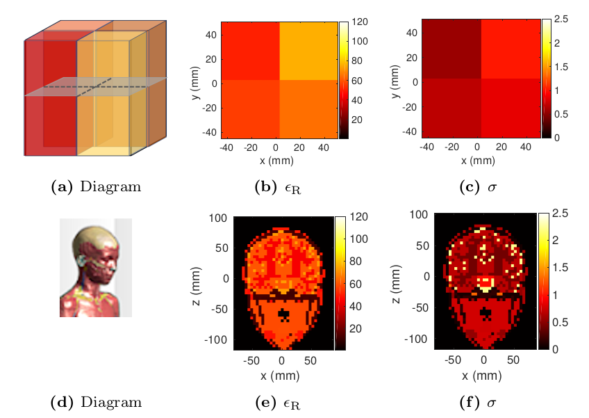
Numerical phantoms and corresponding ground truth of relative permittivity ($$$\epsilon_{\rm R}$$$) and conductivity ($$$\sigma$$$). (a-c) Tissue-Mimicking Four-Compartment Phantom (transverse slice); (d-f) Billie Human-Head Phantom (coronal slice).
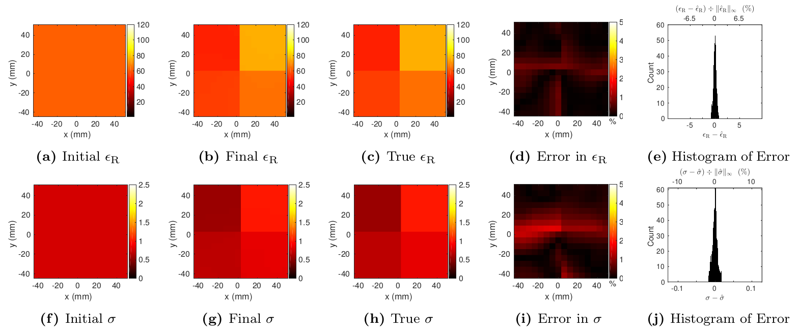
Estimated relative electric permittivity (top) and conductivity (bottom) for the four-compartment phantom at 6mm isotropic resolution, reconstructed from a homogeneous initial guess (a and f) and using $$$b_1^+$$$ measurements with peak SNR of 50. Reconstructed EP are shown for a representative transverse slice through the center of the phantom, at the end of the GMT procedure (b and g). Figs. c and h show the ground truth EP. Figs. d and i show the peak-normalized absolute error. Figs. e and j show the distribution of the error in the final EP over all 4,096 voxels.
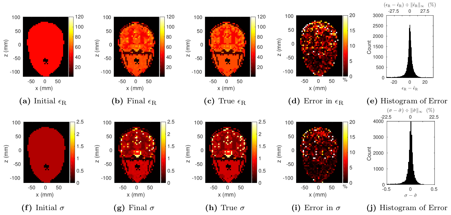
Estimated relative electric permittivity (top) and conductivity (bottom) for the Billie head phantom at 5mm isotropic resolution, reconstructed from a homogeneous initial guess (a and f) and using $$$b_1^+$$$ with peak SNR of 200. Reconstructed EP are shown for a representative coronal slice through the center of the phantom, at the end of the GMT procedure (b and g). Figs. c and h show the ground truth EP. Figs. d and i show the peak-normalized absolute error. Figs. e and j show the distribution of the error in the final EP over all 25,575 voxels.