Introduction

Permittivity mapping strongly depends on the accuracy and the signal-to-noise ratio (SNR) of the underlying B₁⁺ magnitude estimation method. An assessment of different B₁⁺ mapping techniques in the context of permittivity mapping has recently been conducted¹. Another promising candidate, termed B1-TRAP (B₁⁺-mapping with TRAnsient Phase SSFP)², however, has not been investigated so far for its applicability to permittivity mapping. In this work, the B1-TRAP is directly compared to Actual Flip Imaging (AFI) for permittivity mapping in phantom and in vivo.

Methods

The quality of AFI and B1-TRAP for permittivity reconstruction was assessed for in vivo human brain and for a spherical water phantom (relative permittivity = 80) doped with 0.125 mM MnCl₂ to obtain tissue comparable relaxation times (T₁ ~ 870 ms, T₂ ~ 70 ms). For AFI, a non-selective excitation pulse with a flip angle of 45° was used with a TR2 / TR1 = 125 ms / 25 ms, a TE = 4.86 ms, a bandwidth of 120 Hz/Px and an RF phase difference increment of 129.3°. An imaging matrix of 88×64×64 was used, yielding an isotropic voxel size of 2.5 mm. The local flip angle was estimated from the signal ratio $$$r$$$ = S2/S1 and the TR ratio $$$n$$$ = TR2/TR1 = 5 using $$$\alpha\approx\arccos\left[\left(rn-1\right)/\left(n-r\right)\right]$$$. In contrast, B1-TRAP derives the local flip angle directly from the transient FID signal oscillations of steady-state free precession (SSFP). For B1-TRAP, a flip angle of 60° was used for the acquisition of a train of 24 echoes with a bandwidth of 250 Hz/px. In contrast to the AFI, which was acquired in 3D, B1-TRAP acquired 31 interleaved slices (with 100% slice distance) with 2.5 mm in plane resolution and 2.5 mm slice thickness within a TR of 5 s. Two scans were performed, resulting in a total of 62 slices and a resolution similar to the AFI method. The local flip angle was estimated using a dictionary. To this end, the B1-TRAP signal was simulated using the configuration model toolkit³ as a function of the flip angle and over a range of T₁ and T₂ relaxation times. Overall, B₁⁺ mapping with AFI took about 14 minutes and about 11 minutes for B1-TRAP. All scans were carried out on a 3 T clinical MR system (Magnetom Prisma; Siemens Healthcare, Erlangen, Germany) using a 20-channel head coil. Finally, the permittivity was reconstructed from the obtained B₁⁺ maps using⁴:
$$\varepsilon_r\approx-\frac{\nabla^2\left|B_1^+\right|}{\mu\varepsilon_0\omega^2\left| B_1^+\right|}\tag{1}$$
The Laplacian was estimated by local parabola fitting proposed by Katscher et al⁵ and subsequently smoothed with a tissue boundary–preserving median filter⁵. The window size for both the Laplace estimation and the median filter was set to 15×15×15 voxels for the phantom and to 21×21×21 voxels for the brain. For AFI, the TR1 magnitude images, and for the B1-TRAP, the inverted T₂ map, is used as constraint image for the parabola fitting and boundary-preserving median filtering.

Results

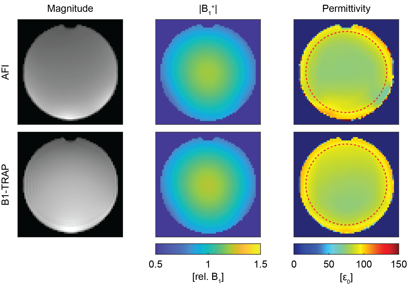
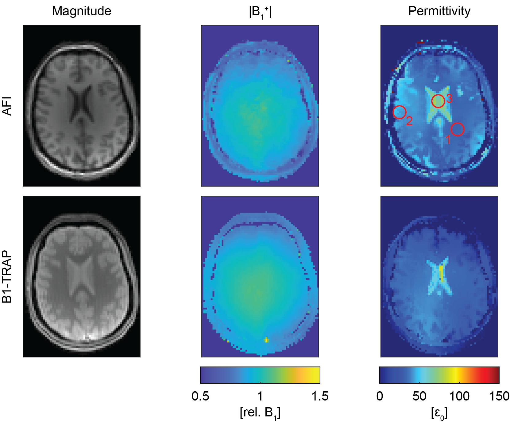
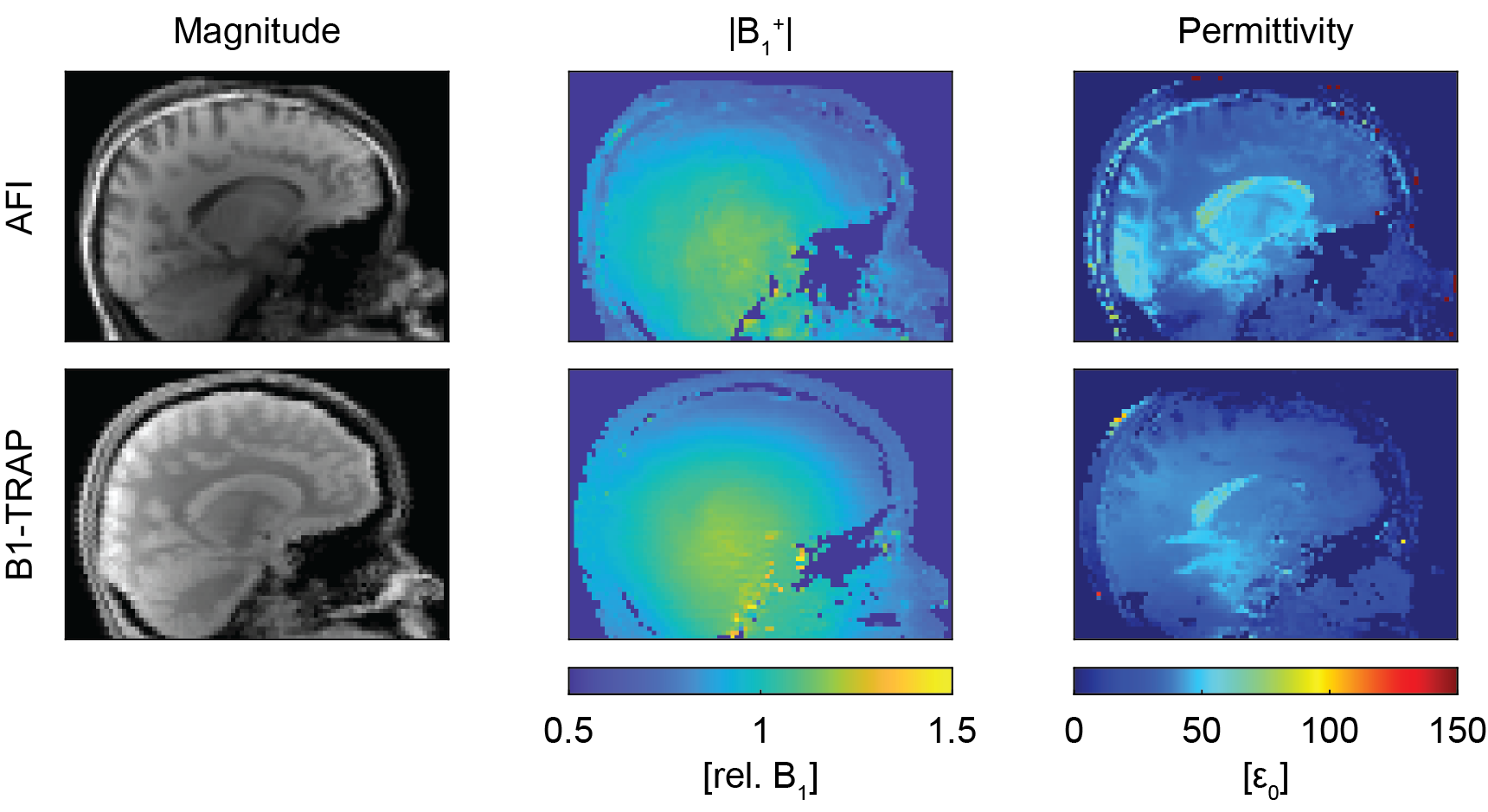
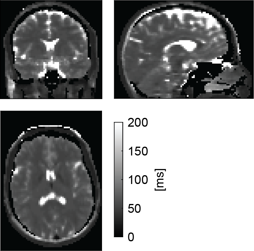
Figure 1 shows for AFI and B1-TRAP an exemplary magnitude slice, together with the corresponding B₁⁺ and the reconstructed permittivity. The AFI permittivity shows a slight inhomogeneity towards the edges of the phantom whereas the permittivity map using B1-TRAP appears more homogenous. For a large region of interest (ROI), relative permittivities of 78.0 ± 4.2 with AFI and 80.6 ± 4.2 with B1-TRAP were found. Figures 2 and 3 show exemplary axial and sagittal images of the in-vivo brain, respectively. Visually, both permittivity maps are of similar quality, but the AFI B₁⁺ map appears to have a higher local variation. Overall, the obtained permittivity values in the brain are underestimated as for relative permittivity values in selected ROIs with AFI yielded 32.2 ± 0.6 for WM, 45.2 ± 1.4 for GM, and 69.5 ± 6.3 for CSF; with B1-TRAP, the values were 32.3 ± 0.4 (WM), 34.7 ± 1.0 (GM), and 62.7 ± 15.6 (CSF). The expected permittivity for WM, GM and CSF are 52, 73 and 84, respectively⁶. The dictionary allowed simultaneous T₂ quantification (see Figure 4), whereas T₁ cannot be reliably estimated.

Discussion

For B1-TRAP, a 2D rather than a 3D approach was used to mitigate any possible motion sensitivity. As a result, a dictionary was used to account for slice profile effects. For the phantom, B1-TRAP yielded improved permittivity homogeneity. For the in-vivo brain, however, although B1-TRAP visually offered increased signal-to-noise in the B₁⁺ map, due to the large Laplacian kernel used, both methods yield similar results and the permittivity is generally underestimated for AFI as well as for B1-TRAP. While B1-TRAP suffers from poor WM/GM differentiation, the higher contrast in the AFI images results in instabilities in the reconstruction that cause areas of noticeable inhomogeneity. In contrast to AFI, B1-TRAP offers the possibility for simultaneous relaxation estimation from the decay of the transient SSFP signal. The decay offered good sensitivity to T₂, whereas T₁ could not reliably estimated.

Conclusion

In conclusion, we showed that B1-TRAP can be used for permittivity mapping in conjunction with T₂ quantification. Paired with a noise-robust reconstruction algorithm, B1-TRAP could be a good candidate for clinical permittivity mapping in vivo at 3 T.

Acknowledgements

This work was supported by the Swiss National Science Foundation (SNF grant No. 325230_182008).