INTRODUCTION

In order to perform a preliminary evaluation of the quality of electric properties tomography (EPT) methods, they are commonly applied to simulated B1-mapping distributions obtained through electromagnetic simulations. This approach has the significant advantage of guaranteeing the knowledge of the ground truth of the electric properties distribution; as a drawback, it does not take into account the effect of artefacts and measurement noise in the performance assessment. To partially overcome this limitation, we propose the adoption of a fast and virtual B1-mapping acquisition that produces synthetic images with a realistic noise distribution starting from the results of electromagnetic simulations. Three B1-mapping techniques are considered: double-angle¹ (DA), actual flip-angle imaging² (AFI) and Bloch–Siegert shift³ (BSS).

METHODS

The virtual acquisitions are obtained by solving the Bloch equations approximately, but coherently with the pulse sequences of the selected B1-mapping techniques. All the considered techniques are based on steady-state gradient-echo (GRE) sequences, whose images are assumed to correspond pixel-by-pixel to the transverse magnetization at the echo time (TE). This assumption allows to avoid simulating the k-space acquisition with the application of gradient fields, reducing the overall computational burden.
The application of a radiofrequency (RF) pulse at each repetition time (TR) is at the heart of the GRE sequences, and so it is the basic ingredient of all computations.
By assuming that the harmonic content of the RF pulse is completely concentrated at the Larmor frequency and that the RF field is purely positively rotating, the RF pulse is modelled by rotating the magnetization around the transverse x-axis of an angle $$$\alpha$$$, rescaled voxel-by-voxel according to the transmit sensitivity $$$|B_1^+|$$$. The actual phase of $$$B_1^+$$$ in each voxel is introduced in the last step, during the synthesis of the image.
After the application of the RF pulse, the magnetization undergoes a relaxation during the whole TR. The longitudinal magnetization is recovered with an exponential trend with time constant T1, whereas the transverse magnetization drops with time constant T2. The considered B1-mapping techniques require a complete spoiling of the transverse magnetization at the end of each TR. This is usually obtained by applying large gradient pulses and changing the phase of the RF pulse at each TR, but their accurate simulation would significantly increase the computational burden; thus, the transverse magnetization is modified artificially at the end of each TR, setting it to a given percentage of its actual value.
Once the steady-state is reached, the transverse magnetization at TE, rescaled by the proton density distribution and the complex receive sensitivity, provides the acquired image.
In addition to alternating rotations and relaxations, the Bloch–Siegert shift technique requires the application of an off-resonance RF pulse, which is simulated by rotating the magnetization around an axis tilted towards the z-axis.
For all the cases, a couple of images are acquired and then combined algebraically to estimate the flip-angle distribution, which is proportional to $$$|B_1^+|$$$. In order to simulate the measurement noise, a Gaussian noise is added to the acquired images before their combination.
The implemented methods are available on github.⁴

RESULTS

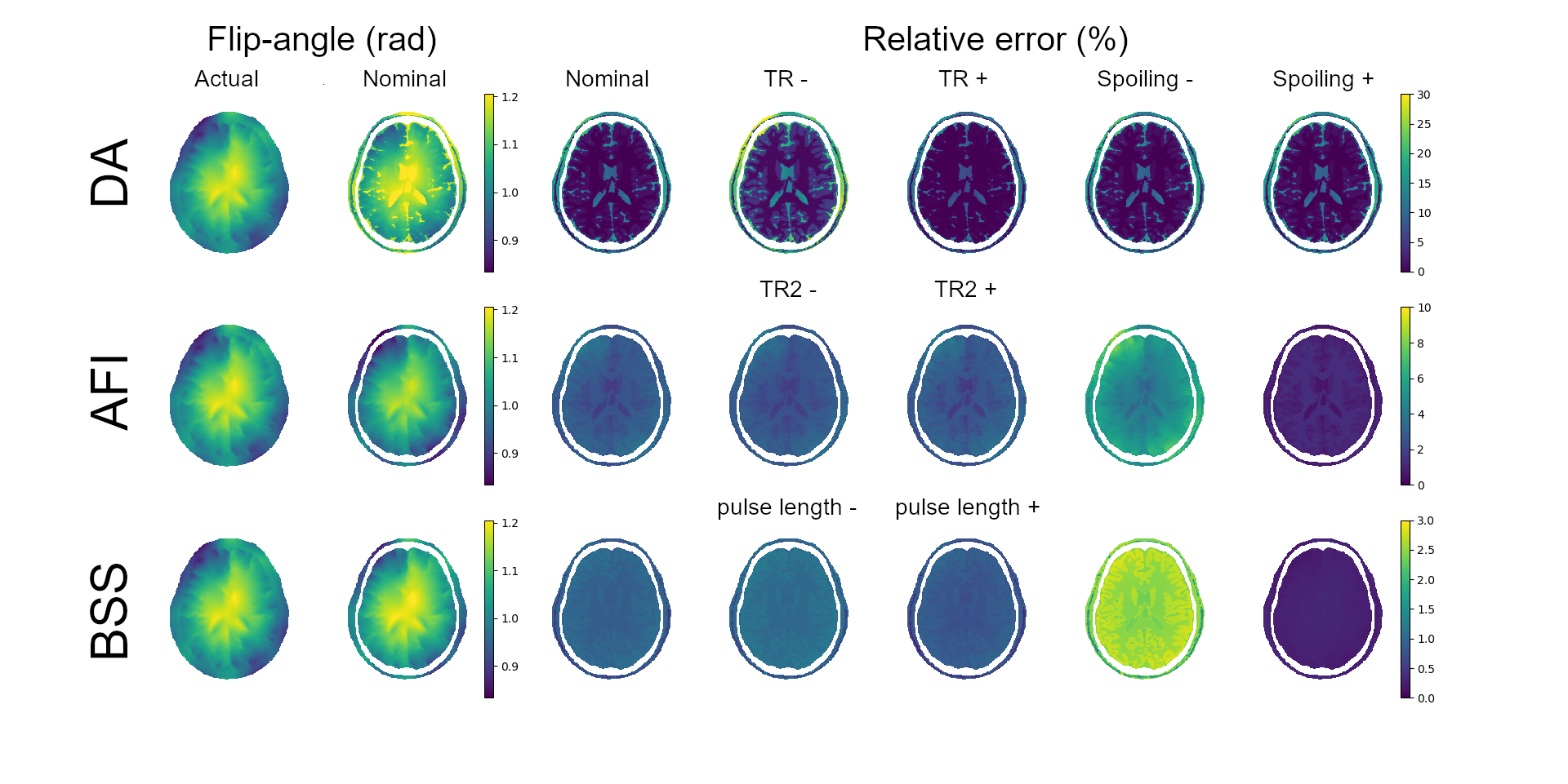
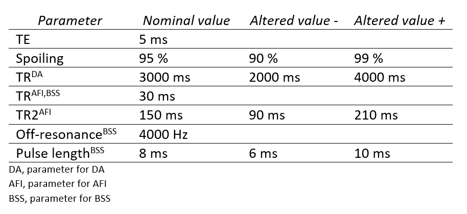
A section of a human head from the BrainWeb database⁵ radiated by an 8-leg birdcage head coil operating at 64 MHz is considered as model problem. The transmit and receive sensitivity of the coil are computed numerically and the first is rescaled to obtain a flip-angle distribution with average $$$\pi/3$$$.
The virtual B1-mapping techniques applied on the simulated data produce the results collected in Figure 1, where the relative error in the estimates is reported as well. The nominal and altered values of the parameters used for each technique are collected in Figure 2.
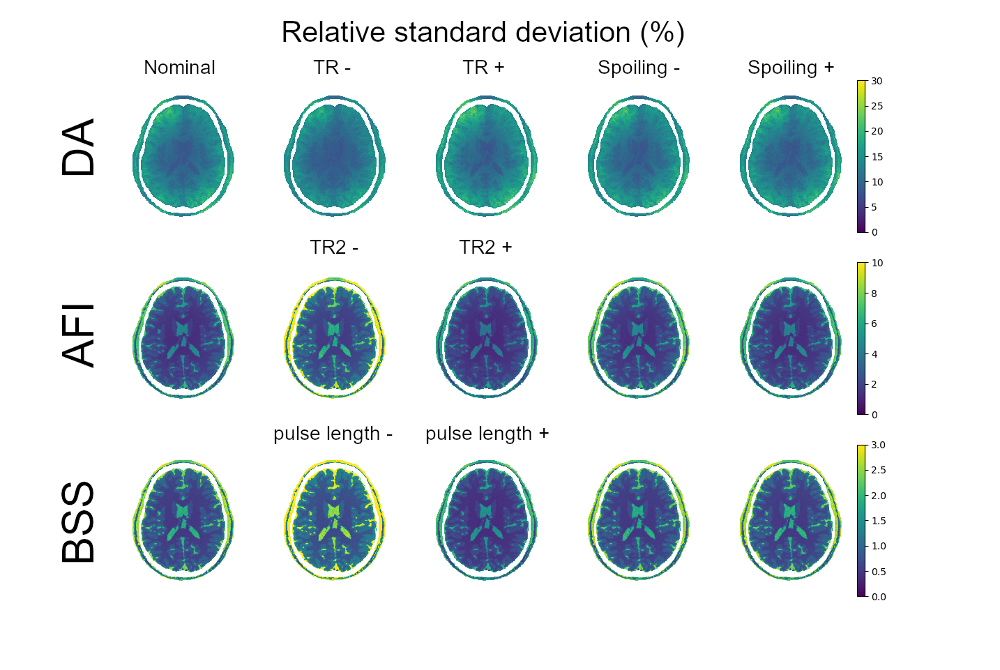
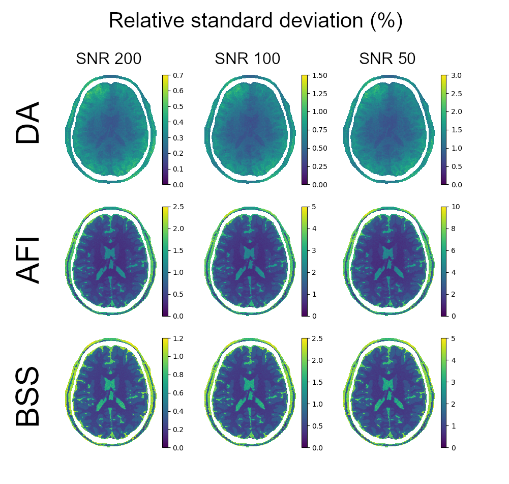
The standard deviation in the flip-angle estimate is evaluated pixel-by-pixel through a Monte Carlo analysis with 100 samples. The results are collected in Figure 3, where the SNR of the images is equal to 200 and the parameters of the techniques are varied, and in Figure 4, where the techniques are applied with nominal parameters and SNR equal to 200, 100 and 50 are considered.
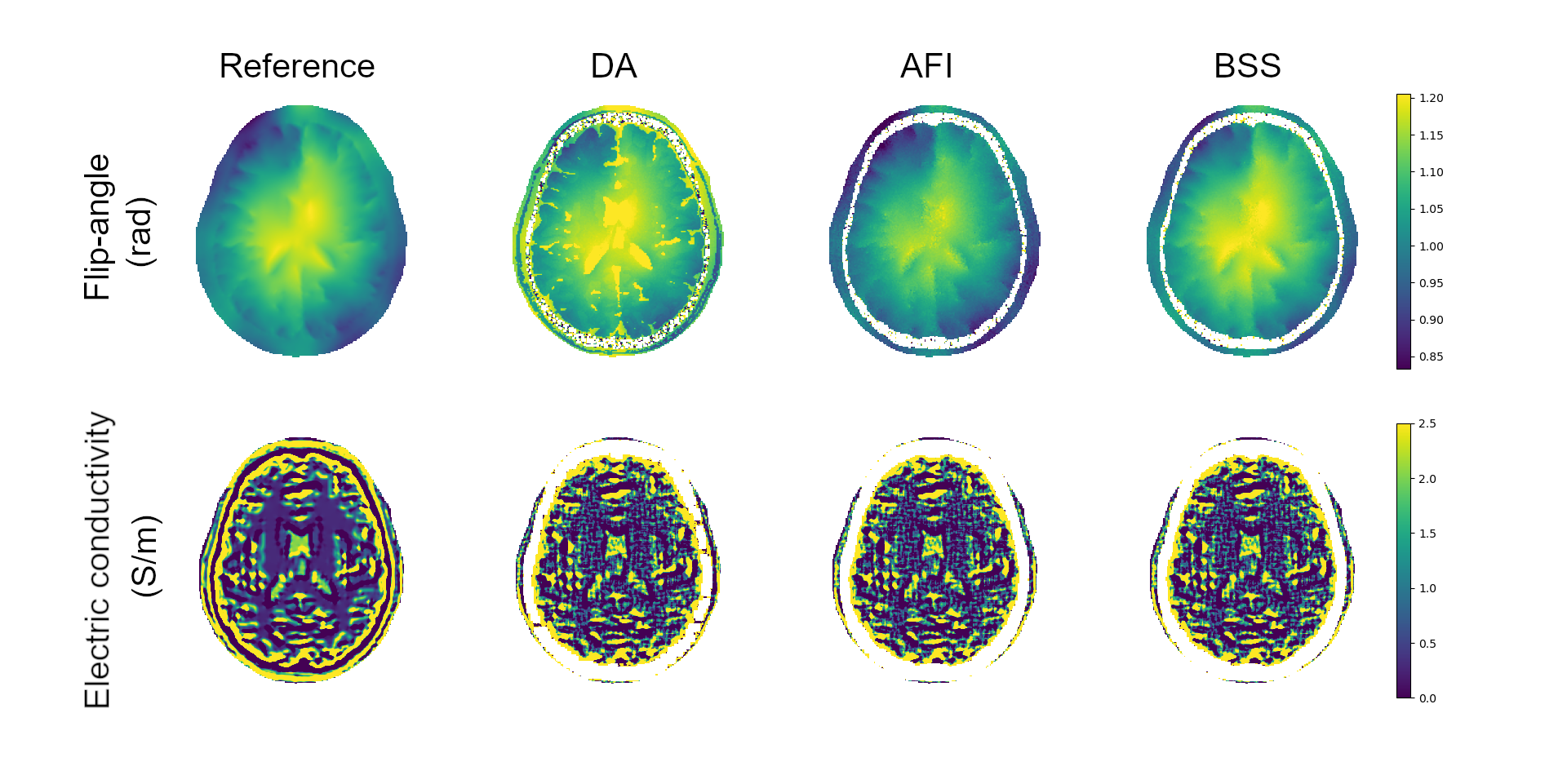
The electric conductivity recovered by applying Helmholtz-EPT to the results of B1-mapping is reported in Figure 5. Helmholtz-EPT implemented in EPTlib⁶ is used with a cubic Savitzky-Golay kernel with $$$n = 2$$$.

DISCUSSION

Although DA is not affected by imperfect spoiling, it introduces large artefacts in tissues with long T1. The error is reduced by increasing the TR.
The errors of AFI and BSS are weakly dependent on the tissue properties. For both the techniques, the quality of the spoiling plays a relevant role in keeping the systematic errors low; whereas the other parameter affects the random errors.
Under the simulated conditions, all the techniques propagate the noise linearly, as evident from Figure 4.
Figure 5 suggests that the errors introduced by the B1-mapping techniques have a small influence in determining the electric conductivity through Helmholtz-EPT.

CONCLUSION

The adoption of fast virtual B1-mapping techniques allows a better understanding of noise propagation through EPT methods by taking into account many realistic features. Nonetheless, the proposed approach could be improved by including the artefacts induced by $$$B_0$$$ inhomogeneities, eddy currents and so on.

Acknowledgements

The results here presented have been developed in the framework of the 18HLT05 QUIERO project. This project 18HLT05 QUIERO has received funding from the EMPIR programme co-financed by the Participating States and from the European Union’s Horizon 2020 research and innovation programme.